# Coherence {#sec-coherence}
[](https://colab.research.google.com/github/{{< var github_user >}}/{{< var repo >}}/blob/main/{{< var subdir >}}/notebooks/coherence.ipynb){.colab-link} Run this chapter's code in Google Colab (no installation).
```{python}
#| include: false
import numpy as np
import matplotlib.pyplot as plt
import pandas as pd
import optolib as ol
ol.use_style()
c0, nm, um = ol.c0, ol.nm, ol.um
```
*Slides 163–171: temporal and spatial coherence, coherence time, coherence length, spectral width, Gaussian pulses.*
## Key relations
A perfect sine wave is perfectly coherent and has a single frequency. A finite wave train of duration $\Delta t$ has a spectrum of
width $\Delta\nu\approx1/\Delta t$ (slides 164–167). Two parts of a beam can only interfere if their path difference is shorter
than the **coherence length**:
$$
\Delta t\approx\frac{1}{\Delta\nu},\qquad l_c=c\,\Delta t=\frac{c}{\Delta\nu}=\frac{\lambda^2}{\Delta\lambda}.
$$
- **Temporal coherence** compares a wave with a delayed copy of itself (slide 166a).
- **Spatial coherence** compares waves emitted from different points of the source (slide 166b).
- For a Gaussian pulse, the FWHM duration and spectral width satisfy $\Delta t\,\Delta\nu\approx0.44$ (slide 167).
::: {.callout-important}
## Convention for $l_c$
The slides use $\Delta t\approx1/\Delta\nu$, hence $l_c=c/\Delta\nu=\lambda^2/\Delta\lambda$. Other definitions include a
line-shape factor. For a Gaussian spectrum with FWHM $\Delta\lambda$, the FWHM of the interferogram envelope (in path difference)
is $(4\ln2/\pi)\,\lambda^2/\Delta\lambda\approx0.88\,\lambda^2/\Delta\lambda$, and the OCT literature quotes half of it,
$(2\ln2/\pi)\,\lambda^2/\Delta\lambda$, as axial resolution. For a Lorentzian line Saleh & Teich use $\tau_c=1/(\pi\Delta\nu)$.
When comparing numbers from different sources, check which definition is used.
:::
### White-light interferogram, live
A Michelson interferometer splits the beam, delays one arm and recombines. Fringes only appear when the optical path difference
(OPD) is shorter than about $l_c$. Broaden the spectrum and watch the fringe packet shrink.
```{ojs}
//| echo: false
viewof co = Inputs.form({
  lam: Inputs.range([400, 1700], {value: 1310, step: 1, label: "centre wavelength λ₀ (nm)"}),
  dl:  Inputs.range([0.5, 300], {value: 50, step: 0.5, label: "spectral width Δλ FWHM (nm)"}),
  span: Inputs.select([20, 50, 100, 200, 1000, 5000], {value: 100, label: "OPD range ± (µm)"})
})
```
```{ojs}
//| echo: false
coData = {
  const k0 = 2*Math.PI/(co.lam*1e-3), dk = 2*Math.PI*(co.dl*1e-3)/((co.lam*1e-3)**2);    // µm⁻¹
  const sig = dk / 2.3548, nk = Math.min(4000, Math.ceil(6*sig / (Math.PI / co.span)) + 101);   // fine enough: no aliasing revival
  const ks = d3.range(nk).map(i => k0 - 3*sig + 6*sig*i/(nk - 1));
  const S = ks.map(k => Math.exp(-4*Math.LN2*((k - k0)/dk)**2)), Ssum = d3.sum(S);
  const N = 2000, out = [];
  for (let i = 0; i <= N; i++) {
    const x = -co.span + 2*co.span*i/N;
    let I = 0;
    for (let j = 0; j < ks.length; j++) I += S[j] * (1 + Math.cos(ks[j]*x));
    out.push({x, I: I / Ssum});
  }
  return out;
}
Plot.plot({
  width: Math.min(width, 1050), height: 280, x: {label: "optical path difference (µm)"}, y: {label: "detector signal", domain: [0, 2.05]},
  marks: [Plot.line(coData, {x: "x", y: "I", stroke: "#2a78d6", strokeWidth: 1})]
})
```
```{ojs}
//| echo: false
{
  const lc = (co.lam*1e-3)**2 / (co.dl*1e-3);
  return html`<div class="result-box">l<sub>c</sub> = λ²/Δλ = <b>${lc.toFixed(1)} µm</b> (slide convention) ·
  envelope FWHM 0.88 λ²/Δλ = ${(0.8825*lc).toFixed(1)} µm · OCT axial resolution (2 ln2/π) λ²/Δλ = ${(0.4413*lc).toFixed(1)} µm in air ·
  Δν = ${(299792.458*co.dl/(co.lam**2)).toFixed(2)} THz</div>`
}
```
If the OPD range is much larger than the fringe packet, the fringes are too dense to draw: zoom in with a smaller range.
## Worked example: sodium lamp and He-Ne laser (slide 168)
```{python}
for name, dnu in (("Na lamp, 589 nm, Δν ≈ 5×10¹¹ Hz", 5e11), ("multimode He-Ne, Δν ≈ 1.5×10⁹ Hz", 1.5e9)):
    lc, dt, _ = ol.coherence_length(dnu=dnu)
    print(f"{name:36s} Δt = {dt:.2e} s, l_c = {lc*1e3:.2f} mm")
```
## Worked example: the exercise of slide 169
```{python}
#| label: tbl-coherence
#| tbl-cap: "Coherence length with the slide convention l_c = c/Δν."
src = [("LED, 1550 nm, Δλ = 150 nm", 1550, ("lam", 150)),
       ("Laser diode, 1550 nm, Δλ = 0.1 nm", 1550, ("lam", 0.1)),
       ("Multimode He-Ne, Δν = 1.5 GHz", 633, ("nu", 1.5e9)),
       ("Single-mode He-Ne, Δν = 10 MHz", 633, ("nu", 10e6)),
       ("Sunlight, 550 nm, Δν ≈ 100 THz", 550, ("nu", 100e12)),
       ("Sodium lamp, 589 nm, Δν ≈ 1 GHz", 589, ("nu", 1e9))]
rows = []
for name, l, (kind, val) in src:
    lc, dt, dnu = ol.coherence_length(wl=nm(l), dlam=nm(val)) if kind == "lam" else ol.coherence_length(dnu=val)
    rows.append({"source": name, "Δν": f"{dnu:.3g} Hz", "Δt": f"{dt:.3g} s",
                 "l_c": f"{lc*1e6:.3g} µm" if lc < 1e-3 else f"{lc:.3g} m"})
pd.DataFrame(rows).set_index("source")
```
The sodium lamp appears twice in the slides with very different widths. Slide 168 uses the whole, pressure-broadened emission
(≈ 5×10¹¹ Hz, 0.6 mm), slide 169 the width of a single Doppler-broadened line (≈ 1 GHz, 30 cm). Both are legitimate. The
coherence length depends on what the instrument actually sees.
## Worked example: fringe visibility and OCT resolution
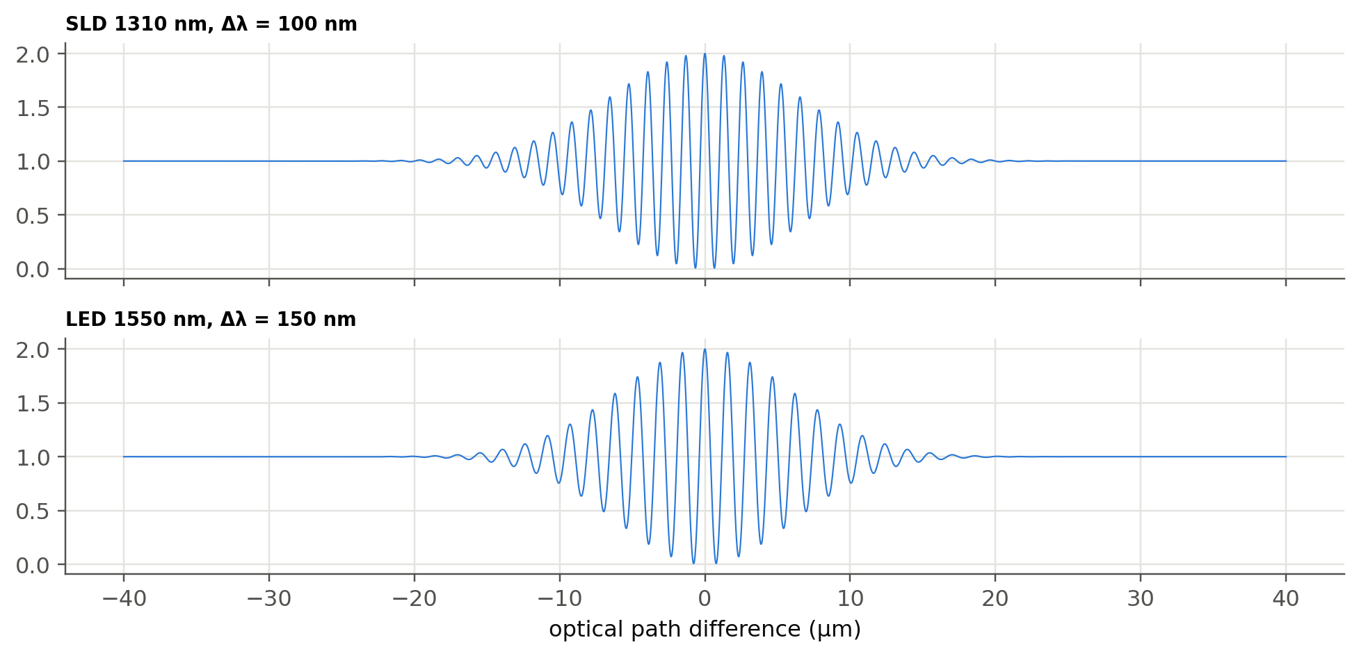
Optical coherence tomography (OCT) exploits low coherence: reflections in tissue are located with a precision of about $l_c/2$.
```{python}
#| label: fig-oct
#| fig-cap: "Michelson interferograms for two broadband sources. The narrower the fringe packet, the better the depth resolution of OCT."
opd = np.linspace(-40e-6, 40e-6, 4000)
fig, ax = plt.subplots(2, 1, figsize=(9, 4.4), sharex=True)
for a, (lbl, l0, dl) in zip(ax, (("SLD 1310 nm, Δλ = 100 nm", nm(1310), nm(100)),
                                 ("LED 1550 nm, Δλ = 150 nm", nm(1550), nm(150)))):
    a.plot(opd*1e6, ol.interferogram(opd, l0, dl), lw=0.7); a.set_title(lbl, fontsize=9, loc="left")
    print(f"{lbl}: OCT axial resolution (Gaussian FWHM) = {2*np.log(2)/np.pi*l0**2/dl*1e6:.1f} µm in air")
ax[1].set_xlabel("optical path difference (µm)"); plt.tight_layout(); plt.show()
```
::: {.callout-tip collapse="true"}
## Going deeper
- Wiener–Khinchin theorem: the degree of temporal coherence $g^{(1)}(\tau)$ is the Fourier transform of the normalised power
spectrum. Verify it numerically with `ol.interferogram`.
- Spatial coherence and the van Cittert–Zernike theorem: why starlight is spatially coherent over a few metres (Michelson stellar
interferometer), and why an LED behind a pinhole can produce fringes.
- Laser linewidth, phase noise and coherent communications: a 100 kHz linewidth laser has $l_c$ of order km. Why do 16-QAM coherent
systems still need carrier-phase recovery?
- Laser speckle is a consequence of high coherence. How is it reduced in laser projectors and LiDAR?
- Coherence length and FMCW LiDAR: what limits the maximum range?
:::
::: {.callout-note collapse="true"}
## Complements
- J. W. Goodman, *Statistical Optics*: the reference for coherence theory.
- Saleh & Teich: chapter "Statistical Optics".
- W. Drexler, J. G. Fujimoto (eds.), *Optical Coherence Tomography: Technology and Applications*.
:::
## Try it yourself
1. A DFB laser has a 1 MHz linewidth. What is its coherence length? Can you build an interferometer with a 1 km arm imbalance?
2. Why can you see colours in a thin soap film (µm) but not in a window pane (mm) under sunlight?
3. Use the live panel to find the spectral width needed for 5 µm OCT resolution at 840 nm.