# Diffraction {#sec-diffraction}
[](https://colab.research.google.com/github/{{< var github_user >}}/{{< var repo >}}/blob/main/{{< var subdir >}}/notebooks/diffraction.ipynb){.colab-link} Run this chapter's code in Google Colab (no installation).
```{python}
#| include: false
import numpy as np
import matplotlib.pyplot as plt
from scipy import special
import optolib as ol
ol.use_style()
c0, nm, um = ol.c0, ol.nm, ol.um
```
*Slides 210–258: Huygens–Fresnel principle, Kirchhoff–Fresnel integral, Arago spot, Fresnel and Fraunhofer regimes, Fraunhofer
diffraction as a Fourier transform, single slit, rectangular and circular apertures (Airy pattern), Rayleigh criterion,
multiple slits, diffraction gratings (Bragg condition, oblique incidence, blazing), wavelength separation.*
## Key relations
Every point of a wavefront is a source of secondary spherical wavelets (Huygens–Fresnel, slides 215–216). Far from an aperture
of size $D$, when $z\gg D$ **and** $z\gg\pi D^2/\lambda$ (slide 222), the diffracted field is the **Fourier transform** of the
aperture (Fraunhofer diffraction, slides 223–225).
| aperture | far-field intensity | first zero | slide |
|---|---|---|---|
| slit of width $a$ | $I(\theta)=I_0\,\mathrm{sinc}^2\beta$, $\ \beta=\tfrac{\pi a\sin\theta}{\lambda}$ | $\sin\theta=\lambda/a$ | 226–232 |
| circular, diameter $D$ | $I(\theta)=I_0\left[\dfrac{2J_1(\gamma)}{\gamma}\right]^2$, $\ \gamma=\tfrac12kD\sin\theta$ | $\sin\theta=1.22\lambda/D$ | 227, 233–235 |
| $N$ slits, period $d$ | slit envelope × $\left[\dfrac{\sin(N\pi d\sin\theta/\lambda)}{\sin(\pi d\sin\theta/\lambda)}\right]^2$ | orders at $d\sin\theta=m\lambda$ | 246–249 |
- **Rayleigh criterion**: two points are just resolved when the Airy peak of one falls on the first zero of the other,
$\sin\Delta\theta_\text{min}=1.22\lambda/D$ (slides 238–239).
- **Grating equation** (slides 248–250): $d(\sin\theta_m-\sin\theta_i)=m\lambda$. Only orders with $|\sin\theta_m|\le1$ propagate.
- **Blazed grating**: the specular reflection on the facets coincides with order $m$ when $2\gamma=\theta_m-\theta_i$ (slides 251, 254).
### Far-field patterns, live
```{ojs}
//| echo: false
viewof df = Inputs.form({
  shape: Inputs.radio(["single slit", "circular aperture", "N slits (grating)"], {value: "single slit", label: "aperture"}),
  a:   Inputs.range([1, 500], {value: 100, step: 1, label: "slit width / diameter (µm)"}),
  lam: Inputs.range([400, 1600], {value: 532, step: 1, label: "wavelength (nm)"}),
  N:   Inputs.range([2, 20], {value: 5, step: 1, label: "number of slits N"}),
  d:   Inputs.range([2, 1000], {value: 300, step: 1, label: "slit period d (µm)"})
})
```
```{ojs}
//| echo: false
dfData = {
  function J1(x) {   // Numerical Recipes rational approximation
    const ax = Math.abs(x);
    if (ax < 8) {
      const y = x*x;
      const a1 = x*(72362614232.0 + y*(-7895059235.0 + y*(242396853.1 + y*(-2972611.439 + y*(15704.48260 + y*(-30.16036606))))));
      const a2 = 144725228442.0 + y*(2300535178.0 + y*(18583304.74 + y*(99447.43394 + y*(376.9991397 + y))));
      return a1/a2;
    }
    const z = 8/ax, y = z*z, xx = ax - 2.356194491;
    const p = 1 + y*(0.183105e-2 + y*(-0.3516396496e-4 + y*(0.2457520174e-5 + y*(-0.240337019e-6))));
    const q = 0.04687499995 + y*(-0.2002690873e-3 + y*(0.8449199096e-5 + y*(-0.88228987e-6 + y*0.105787412e-6)));
    const ans = Math.sqrt(0.636619772/ax)*(Math.cos(xx)*p - z*Math.sin(xx)*q);
    return x < 0 ? -ans : ans;
  }
  const lam = df.lam*1e-3, a = df.a, out = [];
  const thmax = Math.min(Math.asin(Math.min(1, 6*lam/a)) * (df.shape.startsWith("N") ? 1.0 : 1), Math.PI/2);
  const span = df.shape.startsWith("N") ? Math.min(Math.asin(Math.min(1, 3*lam/a)), Math.PI/2) : thmax;
  for (let i = 0; i <= 4000; i++) {
    const th = -span + 2*span*i/4000, s = Math.sin(th);
    let I;
    if (df.shape === "circular aperture") { const g = Math.PI*a*s/lam; I = Math.abs(g) < 1e-9 ? 1 : (2*J1(g)/g)**2; }
    else {
      const b = Math.PI*a*s/lam, env = Math.abs(b) < 1e-9 ? 1 : (Math.sin(b)/b)**2;
      if (df.shape === "single slit") I = env;
      else { const ph = Math.PI*df.d*s/lam, den = Math.sin(ph);
             const arr = Math.abs(den) < 1e-9 ? df.N*df.N : (Math.sin(df.N*ph)/den)**2; I = env*arr/(df.N*df.N); }
    }
    out.push({th: th*1e3, I});
  }
  return out;
}
Plot.plot({
  width: Math.min(width, 1050), height: 300, x: {label: "angle θ (mrad)"}, y: {label: "relative intensity", domain: [0, 1.02], grid: true},
  marks: [Plot.areaY(dfData, {x: "th", y: "I", fill: "#2a78d6", fillOpacity: 0.15}),
          Plot.line(dfData, {x: "th", y: "I", stroke: "#2a78d6", strokeWidth: 1.5})]
})
```
```{ojs}
//| echo: false
{
  const lam = df.lam*1e-3;
  const z1 = df.shape === "circular aperture" ? 1.22*lam/df.a : lam/df.a;
  const far = Math.PI*(df.a*1e-6)**2/(df.lam*1e-9);
  return html`<div class="result-box">first zero at θ = ${(Math.asin(Math.min(1, z1))*1e3).toFixed(2)} mrad
  ${df.shape.startsWith("N") ? ` · grating orders every Δ(sinθ) = λ/d = ${(1e3*lam/df.d).toFixed(2)} mrad, with N − 2 = ${df.N - 2} secondary maxima between them` : ""}
  · Fraunhofer regime for z ≫ πD²/λ = ${far >= 1 ? far.toFixed(2) + " m" : (far*1e3).toFixed(1) + " mm"}</div>`
}
```
## Worked example: Fraunhofer diffraction is an FFT (slides 223–227)
```{python}
#| label: fig-fft
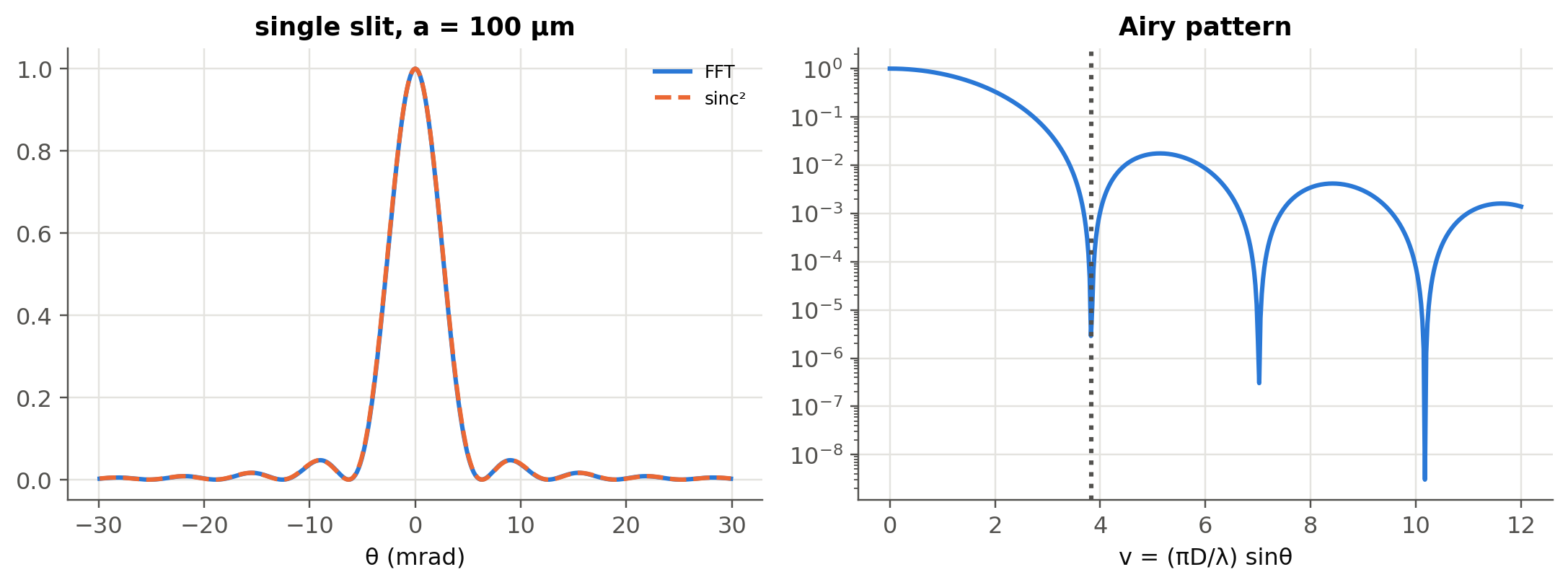
#| fig-cap: "Left: far field of a 100 µm slit computed by FFT and compared with sinc². Right: the Airy pattern [2J₁(v)/v]² of a circular aperture on a log scale; the first zero is at v = 3.83, which gives sinθ = 1.22λ/D."
N, Lw = 4096, 4e-3
x = (np.arange(N) - N//2)*Lw/N
lam, a = nm(633), um(100)
U = (np.abs(x) <= a/2).astype(float)
F = np.fft.fftshift(np.fft.fft(np.fft.ifftshift(U)))
fx = np.fft.fftshift(np.fft.fftfreq(N, Lw/N))
theta = np.arcsin(np.clip(fx*lam, -1, 1))
I_fft = np.abs(F)**2/np.abs(F).max()**2
I_th = np.sinc(a*np.sin(theta)/lam)**2
fig, ax = plt.subplots(1, 2, figsize=(10, 3.8))
sel = np.abs(theta) < 0.03
ax[0].plot(1e3*theta[sel], I_fft[sel], label="FFT"); ax[0].plot(1e3*theta[sel], I_th[sel], "--", label="sinc²")
ax[0].set(xlabel="θ (mrad)", title="single slit, a = 100 µm"); ax[0].legend(fontsize=8)
v = np.linspace(1e-6, 12, 500)
ax[1].semilogy(v, (2*special.j1(v)/v)**2); ax[1].axvline(3.8317, ls=":", c=ol.INK2)
ax[1].set(xlabel="v = (πD/λ) sinθ", title="Airy pattern"); plt.tight_layout(); plt.show()
print(f"Fraunhofer distance for D = 1 mm at 500 nm: πD²/λ = {np.pi*1e-6/500e-9:.1f} m; for D = 10 µm: {np.pi*1e-10/500e-9*1e3:.2f} mm")
```
The last line recomputes slide 222: a 1 mm aperture needs a screen many metres away to be in the Fraunhofer regime, a 10 µm one
less than a millimetre.
```{python}
#| label: fig-rect
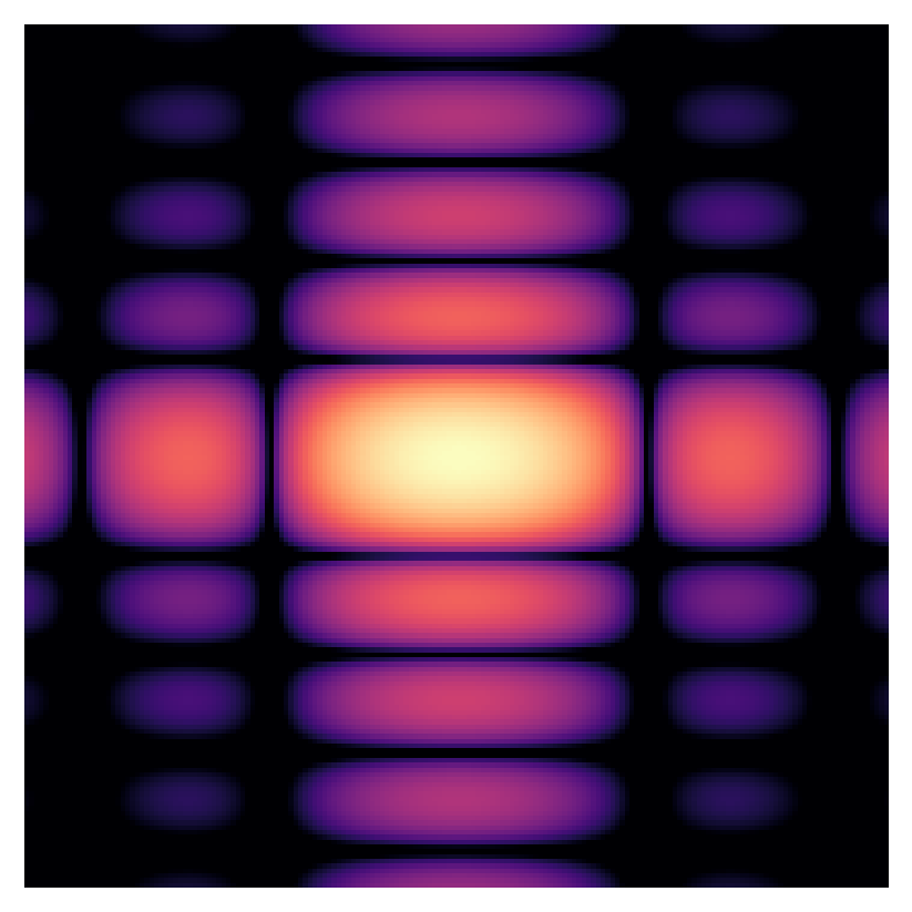
#| fig-cap: "Far-field pattern of a rectangular aperture with b = 2a (slide 236), log scale, from a 2-D FFT."
N2 = 512
x2 = (np.arange(N2) - N2//2)
X, Y = np.meshgrid(x2, x2)
A = ((np.abs(X) <= 6) & (np.abs(Y) <= 12)).astype(float)       # a × b with b = 2a
P = np.abs(np.fft.fftshift(np.fft.fft2(A)))**2
P /= P.max()
fig, ax = plt.subplots(figsize=(4.6, 4.6))
ax.imshow(np.log10(P[N2//2-90:N2//2+90, N2//2-90:N2//2+90] + 1e-5), cmap="magma", vmin=-4); ax.axis("off")
plt.show()
```
The pattern is wider along the *narrow* side of the aperture: diffraction spreads light most where the wave is most constricted.
## Worked example: resolution of the human eye (slide 240)
> Pupil diameter 2 mm, green light 550 nm, eye filled with $n\approx1.33$. What is the minimum angular separation of two points,
> and their separation at 30 cm?
```{python}
dth = np.arcsin(1.22*nm(550)/1.33/2e-3)
s = 2*0.3*np.tan(dth/2)
print(f"Δθ_min = {np.degrees(dth):.4f}°, minimum separation at 30 cm = {s*1e6:.0f} µm (about the thickness of a hair)")
for Nf in (1.8, 2.8, 8):
    print(f"camera at f/{Nf}: Airy radius 1.22 λ N = {1.22*nm(550)*Nf*1e6:.2f} µm (pixel pitch of a phone sensor: 0.8–1.4 µm)")
```
A phone camera at f/1.8 is already close to diffraction-limited at the pixel scale. Shrinking the pixels further gives no extra
resolution, a direct link to the image sensors of Chapter 5.
## Worked example: a reflection grating (slides 253–254)
> $d=10$ µm, $\lambda=1550$ nm, incidence 45°. Find the diffracted beams and the blaze angle. What if $d=2$ µm? What if the
> incidence is 85°?
```{python}
for d, thi in ((um(10), 45), (um(2), 45), (um(10), 85)):
    o = ol.grating_orders(d, nm(1550), thi)
    print(f"d = {d*1e6:.0f} µm, θi = {thi}°: " + ", ".join(f"m = {m:+d}: {t:.1f}°" for m, t in o.items() if abs(m) <= 2))
o = ol.grating_orders(um(10), nm(1550), 45)
print(f"blaze angle for m = +1: γ = (θ1 − θi)/2 = {(o[1] - 45)/2:.1f}°")
```
With $d=10$ µm the first orders are at 59.6° and 33.5° and the blaze angle is 7.3°. With $d=2$ µm, $m=+1$ no longer propagates,
$m=-1$ is at −3.9° and $m=-2$ appears at −57.4°. At 85° incidence the $m=-1$ beam moves to 57.3° (slide: 57.2°) and $m=+1$
disappears, as on slide 254.
## Worked example: separating two wavelengths (slides 255–258)
> A transmission grating with $d=3$ µm, incidence 30°. What is the angular separation of 1550 nm and 1540 nm?
```{python}
o1, o2 = ol.grating_orders(um(3), nm(1550), 30), ol.grating_orders(um(3), nm(1540), 30)
print("propagating orders at 1550 nm:", {m: round(t, 3) for m, t in o1.items()})
for m in sorted(set(o1) & set(o2)):
    if m != 0:
        print(f"order {m:+d}: θ(1550) = {o1[m]:.3f}°, θ(1540) = {o2[m]:.3f}°, separation = {abs(o1[m] - o2[m]):.3f}°")
print(f"periods needed to resolve 0.8 nm (100 GHz DWDM) at 1550 nm in first order: N ≥ λ/Δλ = {1550/0.8:.0f}")
```
At 30° incidence with $d=3$ µm the $m=+1$ order at 1550 nm does not propagate; the $m=-1$ order separates the two wavelengths
by 0.19°. Longer wavelengths are diffracted further, which answers the question of slide 255.
## Worked example: the Arago (Poisson) spot (slides 219–220)
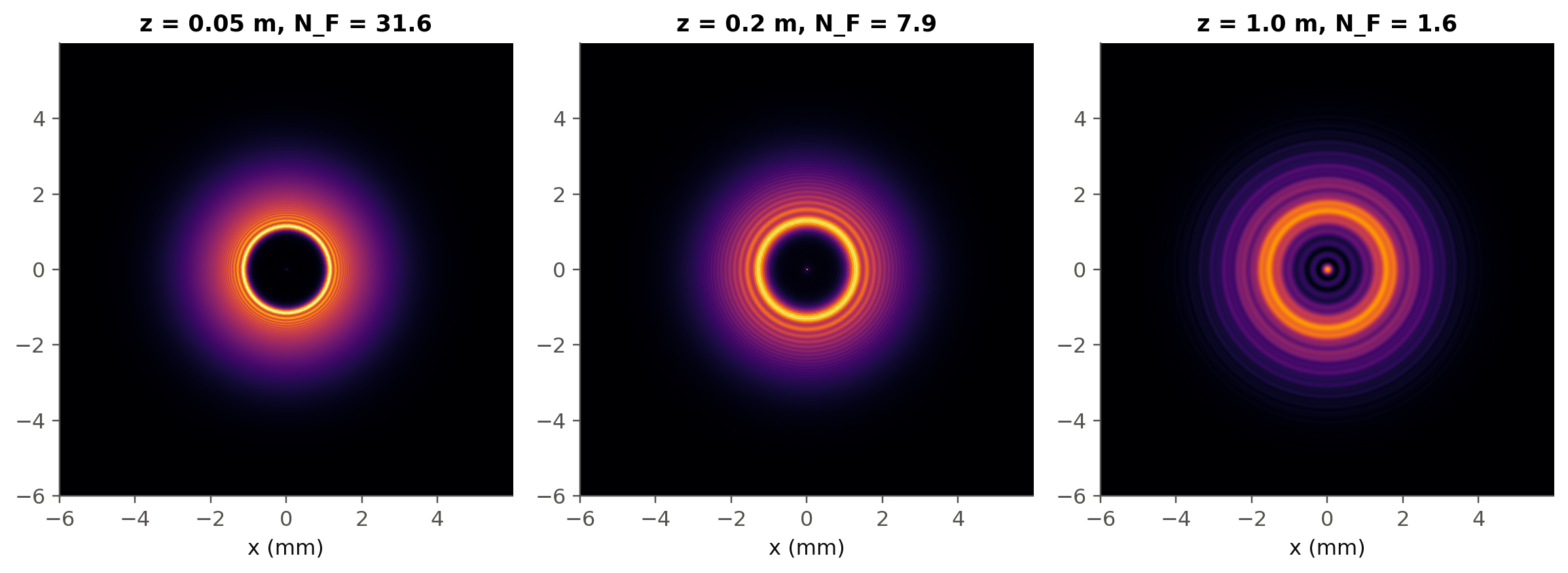
The angular-spectrum method propagates any field by multiplying its 2-D FFT by $e^{-jk_zz}$, with $k_z=\sqrt{k^2-k_x^2-k_y^2}$.
It is the plane-wave superposition of @sec-em made quantitative. A band limit (Matsushima & Shimobaba, 2009) avoids aliasing at
long distances.
```{python}
#| label: fig-arago
#| fig-cap: "A Gaussian beam hitting an opaque 2 mm disc, propagated by the angular-spectrum method. A bright spot appears at the centre of the geometric shadow."
lam, N, Lw = nm(633), 1024, 12e-3
dx = Lw/N; x = (np.arange(N) - N//2)*dx
X, Y = np.meshgrid(x, x); r = np.hypot(X, Y)
a_disk, w_ill = 1e-3, 3e-3
U0 = np.exp(-(r/w_ill)**2)*(r > a_disk)
fig, ax = plt.subplots(1, 3, figsize=(11, 3.8))
for axi, z in zip(ax, (0.05, 0.2, 1.0)):
    I = np.abs(ol.asm_propagate(U0, dx, lam, z))**2
    axi.imshow(I, extent=[x[0]*1e3, x[-1]*1e3]*2, cmap="inferno", vmax=1.0)
    axi.set(title=f"z = {z} m, N_F = {a_disk**2/(lam*z):.1f}", xlabel="x (mm)"); axi.grid(False)
    print(f"z = {z:4.2f} m: on-axis intensity = {I[N//2, N//2]:.3f} "
          f"(incident intensity at the disc rim = {np.exp(-2*(a_disk/w_ill)**2):.3f})")
plt.tight_layout(); plt.show()
```
The bright spot in the shadow has the intensity the beam had at the rim of the disc. Poisson considered this prediction absurd;
Arago observed it (slide 219).
::: {.callout-tip collapse="true"}
## Going deeper
- The Fresnel number $N_F=a^2/(\lambda z)$ decides the regime. Rerun the Arago simulation for $N_F\gg1$ and $N_F\ll1$ and identify
the transition to the far field.
- Talbot effect: a periodic grating self-images at $z_T=2d^2/\lambda$. Demonstrate it with `ol.asm_propagate`.
- A thin lens multiplies the field by $e^{+jkr^2/(2f)}$ (in this convention). Show numerically that the field in its focal plane is
the Fourier transform of the input (4f systems, optical Fourier processing, optical computing).
- Blazed gratings (slide 251): compute the efficiency with a scalar model, and discuss when rigorous (RCWA) models are needed.
- Grating couplers and arrayed-waveguide gratings in silicon photonics are integrated versions of the grating equation: identify
$d$, $\theta_i$ and $\theta_m$ in each.
- Gaussian-beam divergence (@sec-gauss) is itself a diffraction result: compare $\theta=\lambda/(\pi w_0)$ with $1.22\lambda/D$.
:::
::: {.callout-note collapse="true"}
## Complements
- J. W. Goodman, *Introduction to Fourier Optics*: scalar diffraction, angular spectrum, Fresnel and Fraunhofer, optical processing.
- K. Matsushima, T. Shimobaba, "Band-limited angular spectrum method for numerical simulation of free-space propagation in far and
near fields", *Opt. Express* 17, 19662 (2009).
- D. G. Voelz, *Computational Fourier Optics: A MATLAB Tutorial*, SPIE: sampling rules for numerical propagation.
- E. G. Loewen, E. Popov, *Diffraction Gratings and Applications*.
:::
## Try it yourself
1. Use the live panel: double the slit width. What happens to the central lobe? Why does red light give a wider lobe than blue
(slide 245)?
2. The Hubble telescope has a 2.4 m mirror. What is its angular resolution at 500 nm? Could it read a newspaper on the Moon?
3. Design a grating that separates the 100 GHz DWDM channels by 0.1° in first order at 1550 nm.