3 Irradiance and the Poynting vector
 Run this chapter’s code in Google Colab (no installation).
Slides 70–84: magnetic field of the wave, energy density, Poynting vector, average irradiance, spherical waves, power in a Gaussian beam.
3.1 Key relations
The magnetic field always accompanies the electric field, with \(B_y=E_x/v\) and \(v=c/n\) (slide 71). The energy densities of the two fields are equal, so the total energy density is \(\varepsilon_0\varepsilon_rE_x^2\) (slide 73). Energy flows along \(\mathbf k\) with the Poynting vector (slides 74–75):
\[ \mathbf S=v^2\varepsilon_0\varepsilon_r\,\mathbf E\times\mathbf B,\qquad I=\langle S\rangle=\tfrac12 v\,\varepsilon_0\varepsilon_rE_0^2=\tfrac12 c\,\varepsilon_0nE_0^2 . \]
- Detectors are far too slow to follow the optical oscillation (≈ 5 fs period at 1550 nm), so they always measure the average irradiance \(I\) (slide 76).
- A spherical wave spreads its power over \(4\pi r^2\), so \(I=P/(4\pi r^2)\) (slides 77–78).
- A Gaussian beam concentrates its power: \(I_0=2P/(\pi w^2)\) on axis (slides 79–82).
The deep-dive chapter Chapter 15 derives Poynting’s theorem step by step and answers the classic objection: how can energy flow through vacuum, where there is no current?
3.1.1 Field strength from irradiance, live
3.2 Worked example: how strong is the optical field in a fiber and in a chip?
Using \(I=\tfrac12c\,\varepsilon_0nE_0^2\) and, for a Gaussian mode, \(I_0=2P/(\pi w^2)\):
Show the Python
def E0_from_I(I, n): return np.sqrt(2*I/(c0*eps0*n))

cases = [("sunlight at ground (1 kW/m²)", None, 1e3, 1.0),
         ("5 mW He-Ne laser (w = 0.5 mm, slide 83)", (5e-3, 0.5e-3), None, 1.0),
         ("1 mW in SMF-28 (w = 5.2 µm)", (1e-3, um(5.2)), None, 1.444),
         ("100 mW in SMF-28", (100e-3, um(5.2)), None, 1.444),
         ("100 mW in a Si wire (A_eff ≈ 0.1 µm²)", None, 100e-3/0.1e-12, 3.48)]
for name, gauss, I, nn in cases:
    if gauss:
        P, w = gauss; I = 2*P/(np.pi*w**2)
    print(f"{name:42s} I = {I:9.2e} W/m²   E0 = {E0_from_I(I, nn):9.2e} V/m")
sunlight at ground (1 kW/m²) I = 1.00e+03 W/m² E0 = 8.68e+02 V/m
5 mW He-Ne laser (w = 0.5 mm, slide 83) I = 1.27e+04 W/m² E0 = 3.10e+03 V/m
1 mW in SMF-28 (w = 5.2 µm) I = 2.35e+07 W/m² E0 = 1.11e+05 V/m
100 mW in SMF-28 I = 2.35e+09 W/m² E0 = 1.11e+06 V/m
100 mW in a Si wire (A_eff ≈ 0.1 µm²) I = 1.00e+12 W/m² E0 = 1.47e+07 V/mThe silicon-wire case reaches ~\(10^{12}\) W/m² (0.1 GW/cm²) with only 100 mW. This is why two-photon absorption and free-carrier effects appear in silicon photonic circuits at modest powers, and why fiber nonlinearities (Raman, Brillouin; Chapter 14) matter over long distances.
3.3 Spherical waves and the inverse-square law (slides 77–78)
Show the Python
r = np.logspace(-1, 3, 300)
I_bulb = 100/(4*np.pi*r**2)
w, z0 = ol.gaussian_w(r, 0.5e-3, nm(633))
I_laser = 2*5e-3/(np.pi*w**2)
fig, ax = plt.subplots()
ax.loglog(r, I_bulb, label="100 W bulb, I = P/4πr²")
ax.loglog(r, I_laser, label="5 mW He-Ne, on-axis I = 2P/πw²")
ax.axvline(z0, color=ol.INK2, ls=":", lw=1); ax.text(z0*1.1, 1e-3, "z₀", color=ol.INK2)
ax.set(xlabel="distance (m)", ylabel="irradiance (W/m²)"); ax.legend()
plt.show()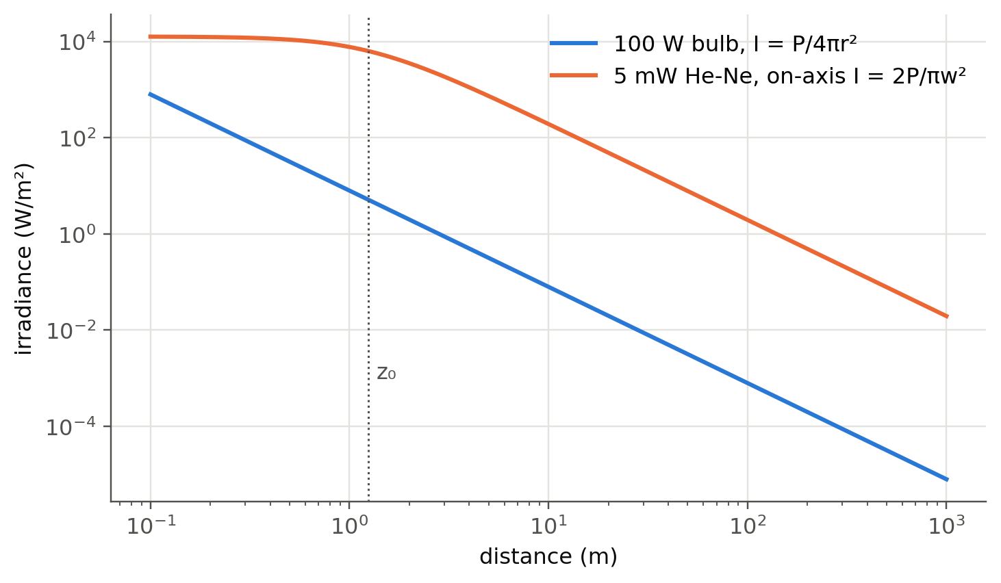
A 5 mW laser is brighter on its axis than a 100 W bulb at any distance shown here. That is why laser safety (IEC 60825-1) is formulated in terms of irradiance, not power.
TipGoing deeper
- Slide 76 notes that detectors only measure time-averaged irradiance. Estimate the optical period at 1550 nm and compare it with the bandwidth of the fastest photodiodes (Chapter 5). What does a coherent receiver measure instead?
- Radiation pressure: \(p=I/c\). Estimate the force of a 1 W beam on a mirror, and relate it to optical tweezers and optomechanics.
- For a guided mode, the power is the integral of \(S_z\) over the cross-section. Why does the “effective area” \(A_\text{eff}\) used in nonlinear optics differ from the geometric core area?
NoteComplements
- D. J. Griffiths, Introduction to Electrodynamics: chapter on electromagnetic waves (energy and momentum).
- Laser-safety standard IEC 60825-1: maximum permissible exposure values are expressed in irradiance.
- Chapter 15, the deep-dive chapter of this book, derives Poynting’s theorem from scratch.
3.4 Try it yourself
- The solar constant above the atmosphere is 1361 W/m². What is the amplitude of the electric field of sunlight?
- A 10 W fiber laser is focused to \(w=10\) µm. Compare the field with the breakdown field of air (~3 MV/m).
- Show that the average energy density of a plane wave, multiplied by its speed \(v\), gives \(I\).