# Fresnel equations, Brewster angle and evanescent waves {#sec-fresnel}
[](https://colab.research.google.com/github/{{< var github_user >}}/{{< var repo >}}/blob/main/{{< var subdir >}}/notebooks/fresnel.ipynb){.colab-link} Run this chapter's code in Google Colab (no installation).
```{python}
#| include: false
import numpy as np
import matplotlib.pyplot as plt
import optolib as ol
ol.use_style()
c0, nm, um = ol.c0, ol.nm, ol.um
```
*Slides 101–147: polarised light, boundary conditions, $r_\perp,r_\parallel,t_\perp,t_\parallel$, internal and external
reflection, Brewster angle, phase change on TIR, evanescent wave, Goos–Hänchen shift, frustrated TIR and beam-splitter cubes,
reflectance and transmittance.*
## Key relations
Resolve the field into components perpendicular ($\perp$, TE) and parallel ($\parallel$, TM) to the plane of incidence
(slide 103). The boundary conditions (continuity of tangential $\mathbf E$ and $\mathbf B$, slides 106–108) give, with
$n=n_2/n_1$, **Fresnel's equations** (slides 110–111):
$$
r_\perp=\frac{\cos\theta_i-\sqrt{n^2-\sin^2\theta_i}}{\cos\theta_i+\sqrt{n^2-\sin^2\theta_i}},\qquad
r_\parallel=\frac{\sqrt{n^2-\sin^2\theta_i}-n^2\cos\theta_i}{\sqrt{n^2-\sin^2\theta_i}+n^2\cos\theta_i},
$$
$$
t_\perp=\frac{2\cos\theta_i}{\cos\theta_i+\sqrt{n^2-\sin^2\theta_i}},\qquad
t_\parallel=\frac{2n\cos\theta_i}{n^2\cos\theta_i+\sqrt{n^2-\sin^2\theta_i}},\qquad
r_\parallel+nt_\parallel=1,\quad r_\perp+1=t_\perp .
$$
| result | formula | slide |
|---|---|---|
| normal incidence | $r=\dfrac{n_1-n_2}{n_1+n_2}$, $\ R=\left(\dfrac{n_1-n_2}{n_1+n_2}\right)^2$ (4 % for glass) | 112, 132 |
| Brewster angle ($r_\parallel=0$) | $\tan\theta_p=n_2/n_1$ | 114–116 |
| TIR phase ($\perp$) | $\tan\dfrac{\phi_\perp}{2}=\dfrac{\sqrt{\sin^2\theta_i-n^2}}{\cos\theta_i}$ | 118 |
| TIR phase ($\parallel$) | $\tan\!\left(\dfrac{\phi_\parallel}{2}+\dfrac{\pi}{2}\right)=\dfrac{\sqrt{\sin^2\theta_i-n^2}}{n^2\cos\theta_i}$ | 119 |
| evanescent field | $E_t\propto e^{-\alpha_2y}$, $\ \alpha_2=\dfrac{2\pi n_2}{\lambda}\sqrt{\left(\dfrac{n_1}{n_2}\right)^2\sin^2\theta_i-1}$ | 123–124 |
| Goos–Hänchen shift | $\Delta z\approx2\delta\tan\theta_i$ | 125 |
| reflectance, transmittance | $R=\lvert r\rvert^2$, $\ T=\dfrac{n_2\cos\theta_t}{n_1\cos\theta_i}\lvert t\rvert^2$, $\ R+T=1$ | 131–138 |
The square root $\sqrt{n^2-\sin^2\theta_i}$ is taken on the branch with non-positive imaginary part. That is the physical choice in
the $e^{j\omega t}$ convention, where the transmitted field decays into medium 2 under TIR. With this choice `ol.fresnel`
reproduces the slide phases.
### Fresnel coefficients, live
```{ojs}
//| echo: false
viewof fr = Inputs.form({
  n1: Inputs.range([1, 4], {value: 1.44, step: 0.01, label: "incidence medium n₁"}),
  n2: Inputs.range([1, 4], {value: 1.00, step: 0.01, label: "second medium n₂"}),
  show: Inputs.radio(["|r| (amplitude)", "R, T (power)", "phase of r"], {value: "|r| (amplitude)", label: "show"})
})
```
```{ojs}
//| echo: false
frData = {
  // small complex helpers
  const C = (re, im = 0) => ({re, im});
  const add = (a, b) => C(a.re + b.re, a.im + b.im), sub = (a, b) => C(a.re - b.re, a.im - b.im);
  const mul = (a, b) => C(a.re*b.re - a.im*b.im, a.re*b.im + a.im*b.re);
  const div = (a, b) => { const d = b.re*b.re + b.im*b.im; return C((a.re*b.re + a.im*b.im)/d, (a.im*b.re - a.re*b.im)/d); };
  const abs = a => Math.hypot(a.re, a.im), arg = a => Math.atan2(a.im, a.re) * 180 / Math.PI;
  const n = fr.n2 / fr.n1, out = [];
  for (let deg = 0; deg <= 89.9; deg += 0.1) {
    const t = deg * Math.PI / 180, ci = C(Math.cos(t)), x = n*n - Math.sin(t)**2;
    const s = x >= 0 ? C(Math.sqrt(x)) : C(0, -Math.sqrt(-x));        // Im ≤ 0 branch
    const n2c = C(n*n*Math.cos(t));
    const rs = div(sub(ci, s), add(ci, s)), rp = div(sub(s, n2c), add(s, n2c));
    const Rs = abs(rs)**2, Rp = abs(rp)**2;
    out.push({deg, v: abs(rs), q: "r⊥"}, {deg, v: abs(rp), q: "r∥"},
             {deg, v: Rs, q: "R⊥"}, {deg, v: Rp, q: "R∥"}, {deg, v: 1 - Rs, q: "T⊥"}, {deg, v: 1 - Rp, q: "T∥"},
             {deg, v: arg(rs), q: "φ⊥"}, {deg, v: arg(rp), q: "φ∥"});
  }
  return out;
}
{
  const keys = fr.show.startsWith("|r|") ? ["r⊥", "r∥"] : fr.show.startsWith("R") ? ["R⊥", "R∥", "T⊥", "T∥"] : ["φ⊥", "φ∥"];
  const thp = Math.atan(fr.n2 / fr.n1) * 180 / Math.PI, thc = fr.n1 > fr.n2 ? Math.asin(fr.n2 / fr.n1) * 180 / Math.PI : null;
  return Plot.plot({
    width: Math.min(width, 1050), height: 330, x: {label: "incidence angle θᵢ (deg)", domain: [0, 90]},
    y: {label: fr.show.startsWith("phase") ? "phase (deg)" : "", grid: true},
    color: {legend: true, domain: keys, range: ["#2a78d6", "#eb6834", "#1baf7a", "#eda100"]},
    marks: [Plot.line(frData.filter(d => keys.includes(d.q) && !d.q.startsWith("T")), {x: "deg", y: "v", stroke: "q", strokeWidth: 2}),
            Plot.line(frData.filter(d => keys.includes(d.q) && d.q.startsWith("T")), {x: "deg", y: "v", stroke: "q", strokeWidth: 2, strokeDasharray: "5,3"}),
            Plot.ruleX([thp], {stroke: "#4a3aa7", strokeDasharray: "3,3"}),
            thc === null ? null : Plot.ruleX([thc], {stroke: "#e34948", strokeDasharray: "3,3"}),
            Plot.tip(frData.filter(d => d.q === keys[0]), Plot.pointerX({x: "deg", y: "v", title: d => `θᵢ = ${d.deg.toFixed(1)}°\n${d.q} = ${d.v.toFixed(3)}`}))]
  });
}
```
```{ojs}
//| echo: false
html`<div class="result-box">${fr.n1 > fr.n2 ? "Internal" : "External"} reflection ·
Brewster angle θp = ${(Math.atan(fr.n2/fr.n1)*180/Math.PI).toFixed(2)}° (violet)
${fr.n1 > fr.n2 ? ` · critical angle θc = ${(Math.asin(fr.n2/fr.n1)*180/Math.PI).toFixed(2)}° (red): beyond it |r| = 1 and only the phase changes` : ""}
· normal incidence R = ${(100*((fr.n1-fr.n2)/(fr.n1+fr.n2))**2).toFixed(2)} %</div>`
```
## Worked example: normal incidence on glass (slides 133–136)
```{python}
for n1, n2, kind in ((1.0, 1.5, "air → glass (external)"), (1.5, 1.0, "glass → air (internal)")):
    rs, rp, ts, tp = ol.fresnel(n1, n2, 0.0)
    print(f"{kind:24s} r = {rs.real:+.2f} ({'180° phase shift' if rs.real < 0 else 'no phase shift'}), R = {abs(rs)**2:.2%}")
print(f"Brewster angle air → glass: θp = {np.degrees(ol.brewster(1, 1.5)):.1f}°  (pile-of-plates polariser, Arago 1812)")
```
## Worked example: reflection and transmission at the Brewster angle (slides 139–141)
```{python}
thp = ol.brewster(1.0, 1.5)
tt = np.arcsin(np.sin(thp)/1.5)
rs, rp, ts, tp = ol.fresnel(1.0, 1.5, thp)
fac = 1.5*np.cos(tt)/np.cos(thp)
print(f"θp = {np.degrees(thp):.2f}°, θt = {np.degrees(tt):.2f}°")
print(f"r⊥ = {rs.real:.3f}, r∥ = {abs(rp):.1e}, t⊥ = {ts.real:.3f}, t∥ = {tp.real:.3f}")
print(f"R⊥ = {abs(rs)**2:.3f}, R∥ = {abs(rp)**2:.1f}, unpolarised R = {abs(rs)**2/2:.3f}")
print(f"T⊥ = {fac*abs(ts)**2:.3f}, T∥ = {fac*abs(tp)**2:.3f}   checks: r∥ + n t∥ = {(rp + 1.5*tp).real:.3f}, r⊥ + 1 = t⊥: {np.isclose(rs + 1, ts)}")
```
The reflected light is purely $\perp$-polarised. The transmitted light is only partially polarised, which is why a stack of
plates is needed to make a good polariser.
## Worked example: TIR between two glasses (slides 142–147)
> $n_1=1.460$, $n_2=1.440$, $\lambda=1300$ nm. Find the critical angle, the phase changes at 87° and 90°, and the penetration depth
> of the evanescent wave.
```{python}
n1, n2, lam = 1.460, 1.440, nm(1300)
print(f"critical angle = {np.degrees(ol.critical_angle(n1, n2)):.2f}°")
for thi in (87, 89.999):
    t = np.radians(thi)
    rs, rp, ts, tp = ol.fresnel(n1, n2, t)
    d = ol.penetration_depth(n1, n2, t, lam)
    print(f"θi = {round(thi)}°: |r⊥| = {abs(rs):.3f}, φ⊥ = {np.degrees(np.angle(rs)):6.1f}°, φ∥ = {np.degrees(np.angle(rp)):6.1f}°, "
          f"α2 = {1/d:.3e} m⁻¹, δ = {d*1e6:.3f} µm" + (f", Goos–Hänchen Δz = 2δ tanθ = {2*d*np.tan(t)*1e6:.1f} µm" if thi < 89 else " (grazing: Δz diverges)"))
```
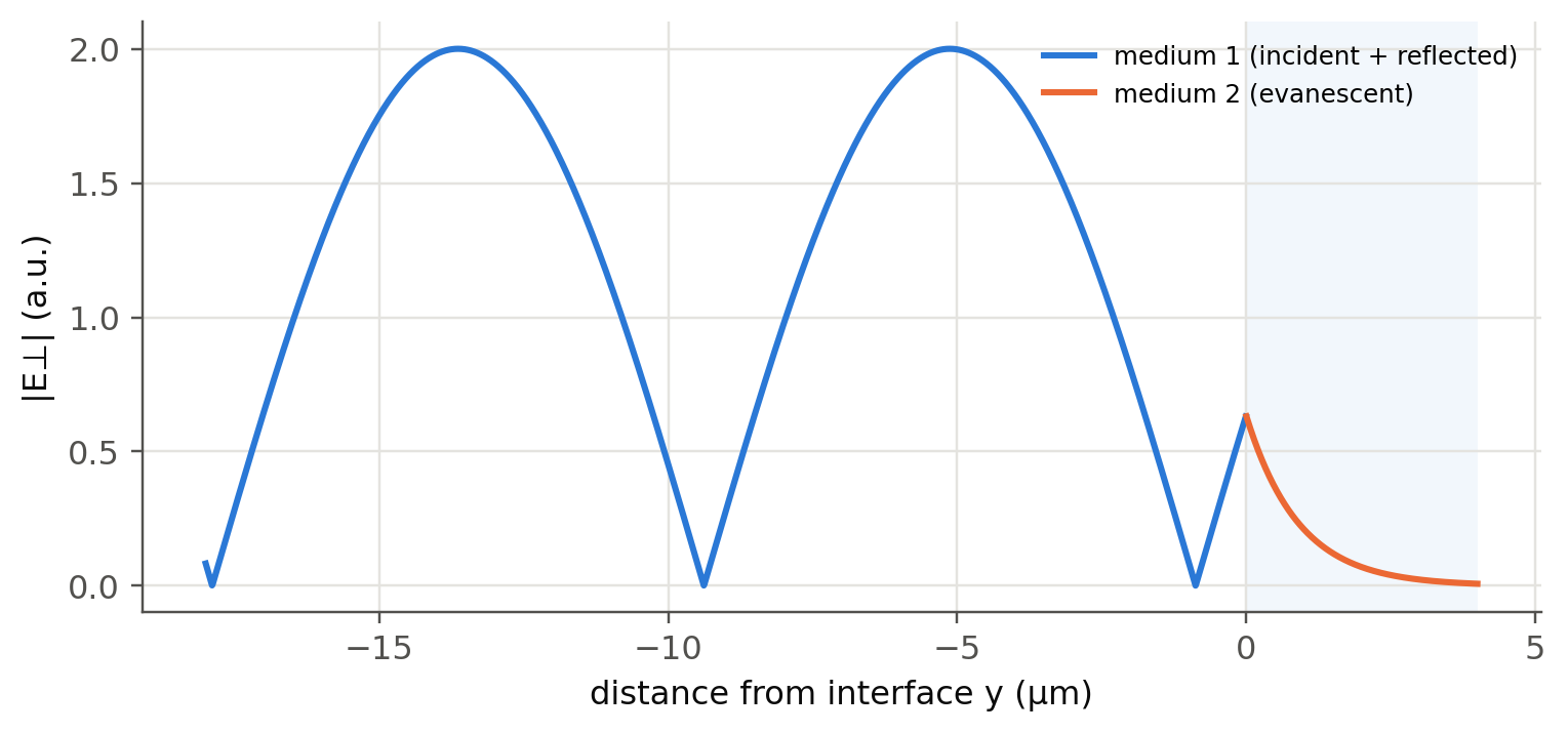
The slides quote $\phi_\perp=143°$, $\phi_\parallel=-36.05°$ (written as $143.95°-180°$), $\delta=0.906$ µm at 87° and 0.859 µm at
90°. The penetration is larger for smaller incidence angles, and it diverges at the critical angle.
```{python}
#| label: fig-evanescent
#| fig-cap: "Field across the interface for TIR at 87° (slide 142 parameters): a standing wave in medium 1 and an exponentially decaying evanescent field in medium 2."
y = np.linspace(-18, 4, 2000)*1e-6
t = np.radians(87)
rs = ol.fresnel(n1, n2, t)[0]
ky = 2*np.pi*n1/lam*np.cos(t)
E1 = np.abs(np.exp(1j*ky*y) + rs*np.exp(-1j*ky*y))          # y < 0: incident + reflected
E2 = np.abs(1 + rs)*np.exp(-y/ol.penetration_depth(n1, n2, t, lam))
fig, ax = plt.subplots(figsize=(8, 3.4))
ax.axvspan(0, 4, color=ol.PALETTE[0], alpha=0.06, lw=0)
ax.plot(y[y < 0]*1e6, E1[y < 0], label="medium 1 (incident + reflected)")
ax.plot(y[y >= 0]*1e6, E2[y >= 0], label="medium 2 (evanescent)")
ax.set(xlabel="distance from interface y (µm)", ylabel="|E⊥| (a.u.)"); ax.legend(fontsize=8)
plt.show()
```
The evanescent tail is exactly what an **evanescent-wave sensor** (ATR spectroscopy, integrated refractive-index sensors) probes,
and what couples two waveguides in a **directional coupler** (Chapter 2).
## Worked example: frustrated TIR, a variable beam splitter (slides 126–129)
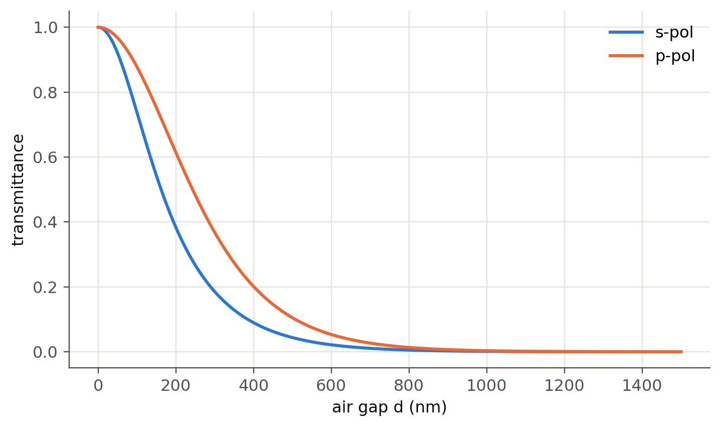
Two glass prisms ($n=1.5$) separated by an air gap, light at 45° (above $\theta_c=41.8°$). When the gap is comparable to the
penetration depth, the evanescent field reaches the second prism and light **tunnels** through. We compute it with the
transfer-matrix solver of @sec-thinfilm.
```{python}
#| label: fig-ftir
#| fig-cap: "Frustrated TIR at 45° and 633 nm: transmittance through an air gap between two glass prisms, for s and p polarisation."
lam = nm(633); gaps = np.linspace(0, 1.5e-6, 300)
fig, ax = plt.subplots()
for pol in ("s", "p"):
    T = [ol.tmm([1.5, 1.0, 1.5], [g], lam, np.radians(45), pol)[1][0] for g in gaps]
    ax.plot(gaps*1e9, T, label=f"{pol}-pol")
ax.set(xlabel="air gap d (nm)", ylabel="transmittance"); ax.legend()
plt.show()
```
A 50/50 splitting ratio requires a gap of a fraction of a wavelength, and the ratio depends on polarisation. This is how the
beam-splitter cube of slide 129 works, and why "polarisation-insensitive" cubes need extra layers. The same tunnelling is used to
couple a laser beam into a thin-film waveguide with a prism (slide 128).
::: {.callout-tip collapse="true"}
## Going deeper
- Derive the Stokes relations $r'=-r$ and $tt'+r^2=1$ from time reversal, and check them numerically with `ol.fresnel`.
- Goos–Hänchen shift (slide 125): the lateral shift is $\propto d\phi/d\theta_i$. Compute it from the phase curves above. Its
transverse counterpart is the Imbert–Fedorov shift (spin Hall effect of light).
- Brewster windows in gas lasers select linear polarisation. Why does a laser with Brewster windows lase in p-polarisation?
- Near $\theta_c$ the penetration depth diverges. What happens for a Gaussian beam with a finite angular spectrum? Use the
plane-wave superposition of @sec-em.
- Verify $R+T=1$ with `ol.tmm` for s and p at oblique incidence, and explain why $T\ne|t|^2$.
:::
::: {.callout-note collapse="true"}
## Complements
- M. Born, E. Wolf, *Principles of Optics*: chapter on the foundations of electromagnetic theory (Fresnel formulae, TIR, evanescent waves).
- H. A. Macleod, *Thin-Film Optical Filters*: characteristic-matrix formulation used by `ol.tmm`.
- N. J. Harrick, *Internal Reflection Spectroscopy*: the classic text on evanescent-wave (ATR) measurements.
:::
## Try it yourself
1. Use the live panel to find the Brewster angle for silicon ($n=3.5$) in air. Why are silicon wafers often inspected with
p-polarised light at that angle?
2. Plot the unpolarised reflectance of a window (two surfaces) versus angle. At which angle is 10 % of the light lost?
3. At which incidence angle does the penetration depth of slide 142 reach 5 µm?