# Gaussian beams {#sec-gauss}
[](https://colab.research.google.com/github/{{< var github_user >}}/{{< var repo >}}/blob/main/{{< var subdir >}}/notebooks/gaussian.ipynb){.colab-link} Run this chapter's code in Google Colab (no installation).
```{python}
#| include: false
import numpy as np
import matplotlib.pyplot as plt
import optolib as ol
ol.use_style()
c0, nm, um = ol.c0, ol.nm, ol.um
```
*Slides 25–34 and 79–84: intensity profile, Rayleigh range, divergence, $M^2$, Gaussian beam in a cavity, power and
irradiance of a Gaussian beam.*
## Key relations
The output of most lasers, and the fundamental mode of a single-mode fiber (slide 27), is a **Gaussian beam**. Its
irradiance across the beam is Gaussian (slides 26, 80):
$$
I(r,z)=\frac{2P}{\pi w^2(z)}\exp\!\left(-\frac{2r^2}{w^2(z)}\right),\qquad
w(z)=w_0\sqrt{1+\left(\frac{z}{z_0}\right)^2},\qquad z_0=\frac{\pi w_0^2 n}{\lambda}.
$$
| quantity | formula | slide |
|---|---|---|
| Rayleigh range (beam area doubled) | $z_0=\pi w_0^2/\lambda$ | 28–29 |
| far-field half-angle divergence | $\theta=\lambda/(\pi w_0)$, total $2\theta$ | 26 |
| real beams | $2\theta=M^2\,\dfrac{4\lambda}{\pi(2w_0)}$, $M^2\ge1$ | 30–31 |
| wavefront radius | $R(z)=z\left[1+(z_0/z)^2\right]$ | 34 |
| Gouy phase | $\psi(z)=\arctan(z/z_0)$ | — |
| power inside radius $w$ | $1-e^{-2}\approx86\,\%$ | 82 |
The complex beam parameter $q(z)=z+jz_0$ (engineering convention: $1/q=1/R-j\lambda/(\pi w^2)$) packs $w$ and $R$ into one
number. It transforms through any paraxial optical system with its $ABCD$ matrix: $q'=(Aq+B)/(Cq+D)$.
### Beam caustic, live
```{ojs}
//| echo: false
viewof gb = Inputs.form({
  w0:  Inputs.range([0.002, 2], {value: 0.5, step: 0.001, label: "waist radius w₀ (mm)"}),
  lam: Inputs.range([0.4, 10.6], {value: 0.633, step: 0.001, label: "wavelength λ (µm)"}),
  M2:  Inputs.range([1, 20], {value: 1, step: 0.1, label: "beam quality M²"}),
  zmax: Inputs.select([0.01, 0.1, 1, 10, 100], {value: 10, label: "plot range (m)"})
})
```
```{ojs}
//| echo: false
gbOut = {
  const w0 = gb.w0 * 1e-3, lam = gb.lam * 1e-6;
  const z0 = Math.PI * w0 * w0 / (gb.M2 * lam);
  const pts = d3.range(-1, 1.0001, 0.002).map(f => {
    const z = f * gb.zmax, w = w0 * Math.sqrt(1 + (z / z0) ** 2);
    return {z, w: w * 1e3, wn: -w * 1e3};
  });
  return {pts, z0, theta: gb.M2 * lam / (Math.PI * w0)};
}
Plot.plot({
  width: Math.min(width, 1050), height: 300, x: {label: "z (m)"}, y: {label: "beam radius (mm)", grid: true},
  marks: [
    Plot.areaY(gbOut.pts, {x: "z", y1: "wn", y2: "w", fill: "#2a78d6", fillOpacity: 0.15}),
    Plot.line(gbOut.pts, {x: "z", y: "w", stroke: "#2a78d6", strokeWidth: 2}),
    Plot.line(gbOut.pts, {x: "z", y: "wn", stroke: "#2a78d6", strokeWidth: 2}),
    Plot.ruleX([-gbOut.z0, gbOut.z0].filter(z => Math.abs(z) <= gb.zmax), {stroke: "#eb6834", strokeDasharray: "4,3"}),
    Plot.ruleY([0], {stroke: "#b9b8b2"}),
    Plot.tip(gbOut.pts, Plot.pointerX({x: "z", y: "w", title: d => `z = ${d.z.toPrecision(3)} m\nw = ${d.w.toPrecision(3)} mm`}))
  ]
})
```
```{ojs}
//| echo: false
html`<div class="result-box">Rayleigh range z₀ = <b>${gbOut.z0 >= 1 ? gbOut.z0.toFixed(2) + " m" : (gbOut.z0*1e3).toFixed(2) + " mm"}</b>
(dashed) · half-angle divergence θ = ${(gbOut.theta*1e3).toFixed(3)} mrad = ${(gbOut.theta*180/Math.PI).toFixed(4)}° ·
beam parameter product w₀θ = ${(gb.w0*gbOut.theta*1e3).toFixed(4)} mm·mrad</div>`
```
## Worked example: power and irradiance of a He-Ne beam (slides 83–84)
> A 5 mW He-Ne laser at 633 nm has a spot size $2w_0=1$ mm. Find the maximum irradiance, and the axial irradiance 25 m away.
```{python}
P, w0, lam = 5e-3, 0.5e-3, nm(633)
I0 = 2*P/(np.pi*w0**2)
w25, z0 = ol.gaussian_w(25, w0, lam)
print(f"I0 = {I0/1e4:.3f} W/cm²,  z0 = {z0:.2f} m")
print(f"at 25 m: 2w = {2*w25*1e3:.1f} mm, axial irradiance = {2*P/(np.pi*w25**2)/1e4*1e3:.2f} mW/cm²")
print(f"fraction of power inside r = w: 1 − e⁻² = {1-np.exp(-2):.3f}")
```
## Worked example: a LiDAR transmitter
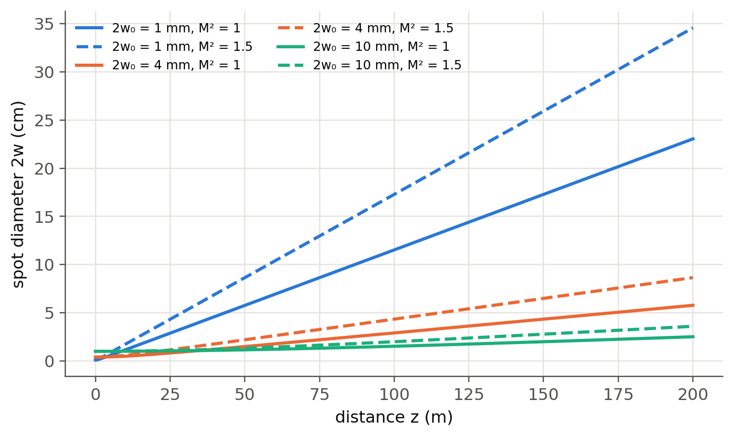
The same formulas size the transmitter of a LiDAR: how large must the output waist be to keep a small footprint at 100 m?
```{python}
#| label: fig-lidar
#| fig-cap: "Spot diameter of a 905 nm LiDAR beam versus distance for three output waists, with ideal (M² = 1, solid) and real (M² = 1.5, dashed) beams. A small waist diverges fast; a large waist stays large."
z = np.linspace(0, 200, 400)
fig, ax = plt.subplots()
for k, w0 in enumerate((0.5e-3, 2e-3, 5e-3)):
    for M2, ls in ((1, "-"), (1.5, "--")):
        ax.plot(z, 2e2*ol.gaussian_w(z, w0, nm(905), M2)[0], ls, color=ol.PALETTE[k],
                label=f"2w₀ = {2e3*w0:.0f} mm, M² = {M2}")
ax.set(xlabel="distance z (m)", ylabel="spot diameter 2w (cm)")
ax.legend(fontsize=8, ncol=2); plt.show()
for zt in (50, 100, 200):
    print(f"optimum waist for range {zt} m: w0 = √(λz/π) = {np.sqrt(nm(905)*zt/np.pi)*1e3:.2f} mm")
```
The optimum waist for a given range $z$ minimises $w(z)$: $w_0^\text{opt}=\sqrt{\lambda z/\pi}$, that is $z=z_0$.
## Worked example: focusing into a single-mode fiber
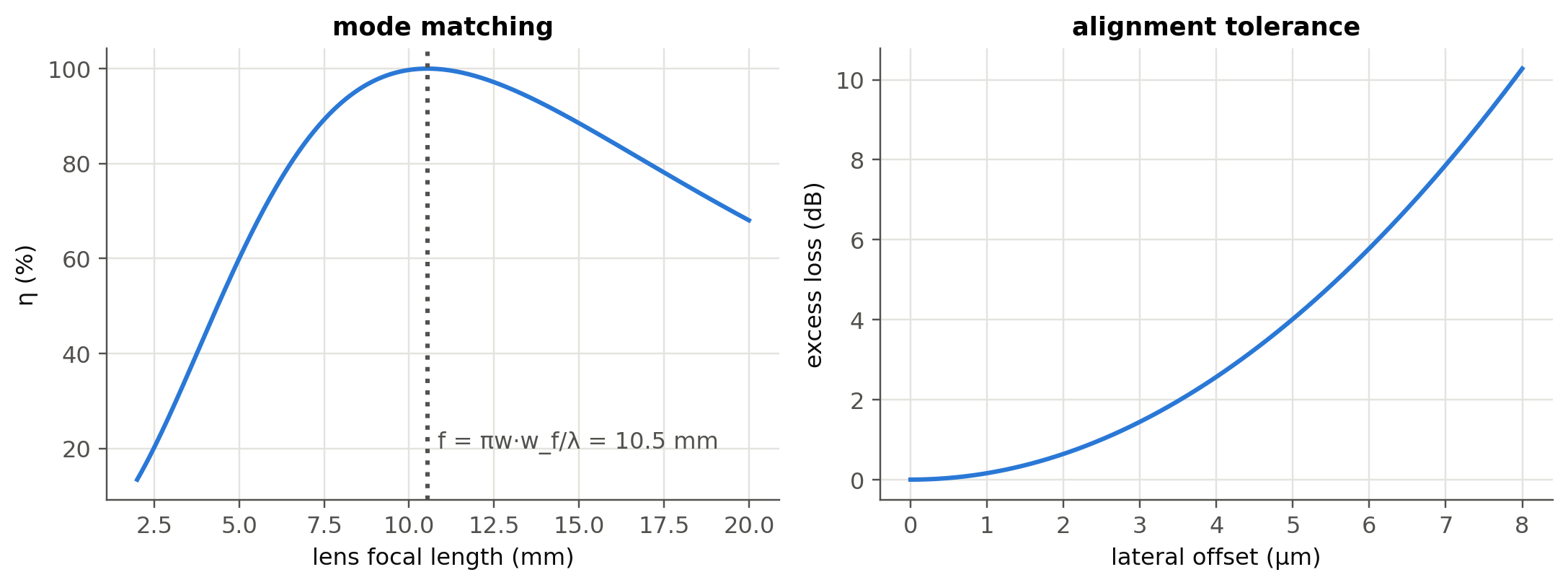
A common laboratory task: couple a collimated 1550 nm beam into an SMF-28 fiber (mode-field diameter ≈ 10.4 µm, so
$w_f\approx5.2$ µm). The fiber mode is well approximated by a Gaussian (slide 27), so the power coupling efficiency between two
Gaussians with waists $w_1, w_2$ and lateral offset $d$ at a common waist plane is
$$
\eta=\left(\frac{2w_1w_2}{w_1^2+w_2^2}\right)^2\exp\!\left(-\frac{2d^2}{w_1^2+w_2^2}\right).
$$
```{python}
#| label: fig-coupling
#| fig-cap: "Left: coupling efficiency into SMF-28 versus the focal length of the coupling lens (1 mm input beam radius). Right: excess loss versus lateral misalignment for perfectly matched waists."
lam, wf, w_in = nm(1550), um(5.2), 1.0e-3
f = np.linspace(2e-3, 20e-3, 300)
w_focus = []
for fi in f:
    q = ol.abcd(ol.q_from_w0(w_in, lam), ol.lens(fi))     # just after the lens
    w_focus.append(ol.w_from_q(ol.abcd(q, ol.free(-np.real(q))), lam))   # new waist where Re(q) = 0
w_focus = np.array(w_focus)
eta = (2*w_focus*wf/(w_focus**2 + wf**2))**2
fig, ax = plt.subplots(1, 2, figsize=(10, 3.8))
ax[0].plot(f*1e3, 100*eta)
f_opt = np.pi*w_in*wf/lam
ax[0].axvline(f_opt*1e3, ls=":", c=ol.INK2)
ax[0].text(f_opt*1e3 + 0.3, 20, f"f = πw·w_f/λ = {f_opt*1e3:.1f} mm", color=ol.INK2)
ax[0].set(xlabel="lens focal length (mm)", ylabel="η (%)", title="mode matching")
d = np.linspace(0, 8e-6, 200)
ax[1].plot(d*1e6, -ol.dB(np.exp(-2*d**2/(2*wf**2))))
ax[1].set(xlabel="lateral offset (µm)", ylabel="excess loss (dB)", title="alignment tolerance")
plt.tight_layout(); plt.show()
```
An offset of 1.5 µm already costs about 0.35 dB. This is why fiber-to-chip packaging is a precision-mechanics problem, and why
silicon photonic chips use spot-size converters (inverse tapers) or grating couplers to enlarge their ~0.5 µm mode.
## Gaussian beam in a cavity (slide 32)
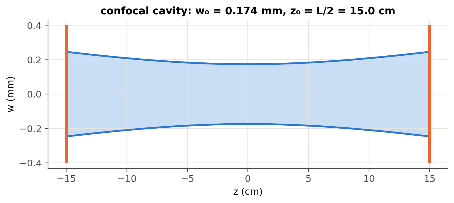
Between two spherical mirrors, the Gaussian beam is a self-consistent solution: the wavefront curvature $R(z)$ matches the
mirror curvature at both ends. For a symmetric **confocal** cavity ($R_\text{mirror}=L$), the waist is $w_0=\sqrt{\lambda L/2\pi}$.
```{python}
#| label: fig-cavity
#| fig-cap: "Gaussian beam inside a symmetric confocal cavity (L = 30 cm, 633 nm). The mirrors (orange) sit where the wavefront radius equals the mirror radius."
L, lam = 0.30, nm(633)
w0 = np.sqrt(lam*L/(2*np.pi)); z0 = np.pi*w0**2/lam
z = np.linspace(-L/2, L/2, 400)
w = w0*np.sqrt(1 + (z/z0)**2)
fig, ax = plt.subplots(figsize=(8, 3))
ax.fill_between(z*100, -w*1e3, w*1e3, color=ol.PALETTE[0], alpha=0.25, lw=0)
ax.plot(z*100, w*1e3, color=ol.PALETTE[0]); ax.plot(z*100, -w*1e3, color=ol.PALETTE[0])
yy = np.linspace(-1.6*w.max()*1e3, 1.6*w.max()*1e3, 50)
for zm, s in ((L/2, 1), (-L/2, -1)):
    ax.plot((zm - s*(L - np.sqrt(L**2 - (yy*1e-3)**2)))*100, yy, color=ol.PALETTE[1], lw=3)
ax.set(xlabel="z (cm)", ylabel="w (mm)", title=f"confocal cavity: w₀ = {w0*1e3:.3f} mm, z₀ = L/2 = {z0*100:.1f} cm")
plt.show()
```
## Measuring $M^2$ in the lab (optional package)
```{python}
#| eval: false
# pip install laserbeamsize   (ISO 11146 beam-width and M² fitting)
import laserbeamsize as lbs
# images: list of camera frames recorded at positions z (m) along the caustic
d = np.array([lbs.beam_size(img)[2] for img in images]) * pixel_size
params, errors, used = lbs.M2_fit(z, d, nm(633))
d0, z0_pos, theta, M2, zR = params     # waist diameter, waist position, full divergence, M², Rayleigh distance
```
::: {.callout-tip collapse="true"}
## Going deeper
- Why is the "86 % power" diameter $2w$ (slide 82)? Integrate the Gaussian and show that the fraction inside $r=w$ is $1-e^{-2}$.
- The **Gouy phase** $\psi(z)$ is missing from the slide formulas. It shifts the resonance frequencies of transverse modes in a
spherical-mirror cavity (slide 32): $\nu_{mnq}=\frac{c}{2nL}\left[q+(m+n+1)\frac{\Delta\psi}{\pi}\right]$. Look up Hermite–Gaussian
modes and explain why a confocal cavity is degenerate.
- $M^2$ can be defined from second moments of the intensity (ISO 11146). Why do the second moments fail for a top-hat beam
with hard edges (sinc² far field)?
- The beam parameter product $w_0\theta=M^2\lambda/\pi$ is invariant through lossless optics (étendue). Relate it to the brightness
theorem and to why an LED cannot be focused into a single-mode fiber efficiently (Chapter 3).
- Fiber modes are only approximately Gaussian. The Marcuse formula $w/a\approx0.65+1.619V^{-3/2}+2.879V^{-6}$ links $w$ to the
normalised frequency $V$ of Chapter 2.
:::
::: {.callout-note collapse="true"}
## Complements
- A. E. Siegman, *Lasers*: chapters on Gaussian beams, ABCD matrices and beam quality. The reference text.
- Saleh & Teich, chapter "Beam Optics" (Gaussian and Hermite–Gaussian beams, ABCD law).
- ISO 11146-1: test methods for laser beam widths, divergence angles and beam propagation ratios.
:::
## Try it yourself
1. Check numerically that $w_0^\text{opt}=\sqrt{\lambda z/\pi}$ minimises $w(z)$ at a given distance.
2. A green laser pointer (532 nm, 1 mm beam, M² = 1.2) is aimed at the Moon (384 000 km). How large is the spot?
3. Extend the fiber-coupling cell to include an axial (focus) error. Which is more critical, 10 µm of defocus or 1 µm of offset?