# Optical resonators: the Fabry–Perot cavity {#sec-fp}
[](https://colab.research.google.com/github/{{< var github_user >}}/{{< var repo >}}/blob/main/{{< var subdir >}}/notebooks/fabry-perot.ipynb){.colab-link} Run this chapter's code in Google Colab (no installation).
```{python}
#| include: false
import numpy as np
import matplotlib.pyplot as plt
import pandas as pd
import optolib as ol
ol.use_style()
c0, nm, um = ol.c0, ol.nm, ol.um
```
*Slides 191–209: cavity modes, free spectral range, finesse, mode linewidth, Q-factor, etalons, scanning Fabry–Perot
interferometer, mirror requirements, worked examples.*
## Key relations
Two parallel mirrors of reflectance $R$ separated by $L$ trap light. The circulating field is the sum of all round trips
(slide 194), $E_\text{cavity}=A+Ar^2e^{-j2kL}+Ar^4e^{-j4kL}+\dots$, which peaks when $k_mL=m\pi$. The allowed standing waves are
the **cavity modes** (slides 193–196):
$$
m\frac{\lambda_m}{2}=nL,\qquad \nu_m=m\frac{c}{2nL},\qquad \nu_f=\frac{c}{2nL}\ \text{(free spectral range)},
$$
$$
\mathcal F=\frac{\pi\sqrt R}{1-R},\qquad \delta\nu_m=\frac{\nu_f}{\mathcal F},\qquad Q=\frac{\nu_m}{\delta\nu_m}=m\mathcal F .
$$
The cavity is also a **filter**: only its modes are transmitted (slide 198). A lossless cavity has the Airy transmission
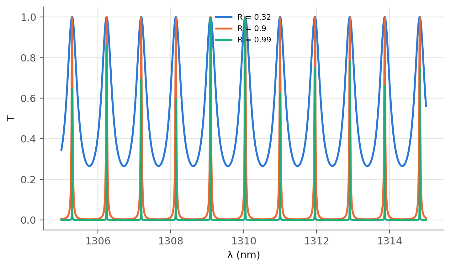
$T=\dfrac{(1-R)^2}{(1-R)^2+4R\sin^2(2\pi nL/\lambda)}$. For a finesse above about 100, only multilayer dielectric mirrors (@sec-bragg)
are good enough (slide 204).
### Airy function, live
```{ojs}
//| echo: false
viewof fp = Inputs.form({
  R: Inputs.range([0.04, 0.995], {value: 0.9, step: 0.005, label: "mirror reflectance R"}),
  L: Inputs.range([1, 1000], {value: 100, step: 1, label: "cavity length L (µm)"}),
  n: Inputs.range([1, 4], {value: 1, step: 0.01, label: "refractive index n"}),
  l0: Inputs.range([400, 1700], {value: 900, step: 1, label: "centre wavelength (nm)"})
})
```
```{ojs}
//| echo: false
fpOut = {
  const fsr_nm = fp.l0**2 / (2*fp.n*fp.L*1000), span = Math.max(3*fsr_nm, 0.02);
  const data = [];
  for (let i = 0; i <= 3000; i++) {
    const l = fp.l0 - span/2 + span*i/3000;
    const s = Math.sin(2*Math.PI*fp.n*fp.L*1000/l);
    data.push({l, T: (1 - fp.R)**2 / ((1 - fp.R)**2 + 4*fp.R*s*s)});
  }
  const F = Math.PI*Math.sqrt(fp.R)/(1 - fp.R), fsr = 299792458/(2*fp.n*fp.L*1e-6);
  const m = Math.round(2*fp.n*fp.L*1000/fp.l0);
  return {data, F, fsr, fsr_nm, m, Q: m*F, dnu: fsr/F};
}
Plot.plot({
  width: Math.min(width, 1050), height: 300, x: {label: "λ (nm)"}, y: {label: "transmission T", domain: [0, 1.02], grid: true},
  marks: [Plot.line(fpOut.data, {x: "l", y: "T", stroke: "#2a78d6", strokeWidth: 2}),
          Plot.tip(fpOut.data, Plot.pointerX({x: "l", y: "T", title: d => `λ = ${d.l.toFixed(3)} nm\nT = ${d.T.toFixed(3)}`}))]
})
```
```{ojs}
//| echo: false
html`<div class="result-box">FSR = ${(fpOut.fsr/1e9).toFixed(1)} GHz = ${fpOut.fsr_nm.toFixed(3)} nm · finesse 𝓕 = <b>${fpOut.F.toFixed(1)}</b> ·
mode linewidth δν = ${(fpOut.dnu/1e9).toFixed(3)} GHz · mode number m ≈ ${fpOut.m} · Q = m𝓕 ≈ <b>${fpOut.Q.toExponential(2)}</b></div>`
```
## Worked examples (slides 205–209), recomputed
> (a) A cavity in air, $L=100$ µm, $R=0.90$. Find the mode nearest to 900 nm, the mode separation, finesse, linewidth and $Q$.
> (b) A semiconductor cavity, $L=250$ µm, $n=3.6$, $R=0.90$, near 1310 nm.
```{python}
#| label: tbl-fp
#| tbl-cap: "Fabry–Perot cavities of slides 205–209, plus a laser-diode cavity with cleaved facets."
tab = pd.DataFrame({
    "air, 100 µm, R = 0.9, 900 nm (slides 205–206)": ol.fp_summary(um(100), 1.0, 0.90, nm(900)),
    "semiconductor, 250 µm, n = 3.6, R = 0.9, 1310 nm (slides 207–209)": ol.fp_summary(um(250), 3.6, 0.90, nm(1310)),
    "same, cleaved facets R = ((n−1)/(n+1))²": ol.fp_summary(um(250), 3.6, ((3.6-1)/4.6)**2, nm(1310))}).T
tab.columns = ["m", "λ_m (nm)", "ν_m (THz)", "FSR (GHz)", "FSR (nm)", "finesse", "δν (GHz)", "δλ (nm)", "Q"]
tab.round(3)
```
The slides give $m=222$, $\lambda_m=900.90$ nm, $\nu_f=1.5$ THz, $\mathcal F=29.8$ and $Q=6.6\times10^3$ for (a), and $m=1374$,
$\nu_f=1.67\times10^{11}$ Hz and $Q=4.1\times10^4$ for (b). The last row replaces the slide's $R=0.9$ by the Fresnel reflectance of a
cleaved facet (@sec-fresnel): this is the "cold" cavity of a Fabry–Perot laser diode, whose longitudinal modes (≈ 0.95 nm apart
here) you will see in the optical spectrum of the lab laser.
```{python}
#| label: fig-airy
#| fig-cap: "Airy transmission of a lossless semiconductor cavity (n = 3.6, L = 250 µm) for three mirror reflectances. R = 0.32 is a cleaved facet."
lam = np.linspace(nm(1305), nm(1315), 4000)
fig, ax = plt.subplots()
for R in (0.32, 0.9, 0.99):
    ax.plot(lam*1e9, ol.airy_T(lam, um(250), R, 3.6), label=f"R = {R}")
ax.set(xlabel="λ (nm)", ylabel="T"); ax.legend(fontsize=8); plt.show()
```
## Scanning Fabry–Perot spectrum analyser (slides 202–203)
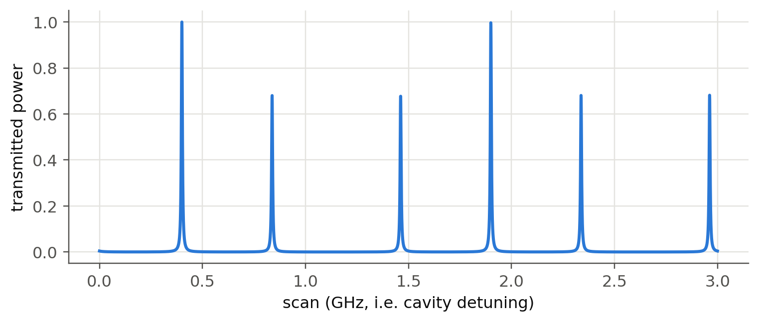
A confocal scanning interferometer with FSR = 1.5 GHz and finesse 250 resolves lines $1.5\ \text{GHz}/250=6$ MHz apart (the
datasheet quotes 7.5 MHz). Scanning the length with a piezo sweeps every mode through one FSR. Here it resolves the longitudinal
modes of a He-Ne laser:
```{python}
#| label: fig-scan
#| fig-cap: "Simulated scan of a He-Ne laser (three longitudinal modes 438 MHz apart under a Doppler gain envelope) with a 1.5 GHz FSR, finesse-250 analyser."
fsr, F = 1.5e9, 250
nu_scan = np.linspace(0, 2*fsr, 6000)
modes = np.array([-438e6, 0, 438e6]) + 0.4e9
amps = np.exp(-(modes - 0.4e9)**2/(2*(500e6)**2))
sig = sum(a/(1 + (2*F/np.pi)**2*np.sin(np.pi*(nu_scan - m)/fsr)**2) for a, m in zip(amps, modes))
fig, ax = plt.subplots(figsize=(8, 3))
ax.plot(nu_scan/1e9, sig); ax.set(xlabel="scan (GHz, i.e. cavity detuning)", ylabel="transmitted power")
plt.show()
```
::: {.callout-tip collapse="true"}
## Going deeper
- Photon lifetime and linewidth: show that $\delta\nu=1/(2\pi\tau_{ph})$ and relate $\tau_{ph}$ to the mirror loss
$\alpha_m=\frac{1}{2L}\ln\frac{1}{R_1R_2}$. This mirror loss is the threshold gain of the laser in Chapter 4.
- Add internal loss (or gain) to the Airy function. When does the transmission peak exceed 1? What does that mean physically
(regenerative amplification)?
- The microring resonator is the integrated-photonics equivalent of the Fabry–Perot cavity: derive its FSR, finesse and $Q$ from
coupling and loss, and compare critical coupling with impedance matching.
- Why do high-finesse cavities need dielectric mirrors (slide 204)? Link it to absorption in metals (@sec-index).
- The same Airy curves come out of the transfer-matrix solver if you put two Bragg mirrors around a spacer layer, with an extra
phase from the mirror penetration depth (@sec-bragg).
:::
::: {.callout-note collapse="true"}
## Complements
- Saleh & Teich: chapter "Resonator Optics".
- W. Bogaerts *et al.*, "Silicon microring resonators", *Laser Photonics Rev.* 6, 47 (2012).
- Siegman, *Lasers*: optical resonators and mode frequencies (with the Gouy phase, @sec-gauss).
:::
## Try it yourself
1. Use the live panel to design a 100 GHz-FSR etalon in fused silica ($n=1.444$). How thick is it? What reflectance gives a
10 GHz linewidth?
2. What is the minimum finesse needed to resolve the He-Ne modes in the scan figure? Check by changing `F`.
3. A VCSEL has a cavity only one wavelength long. Estimate its FSR and explain why it is single-longitudinal-mode.