# The diode: forward and reverse bias {#sec-diode}
[](https://colab.research.google.com/github/{{< var github_user >}}/{{< var repo >}}/blob/main/{{< var subdir >}}/notebooks/diode.ipynb){.colab-link} Run this chapter's code in Google Colab (no installation).
```{python}
#| include: false
import numpy as np
import matplotlib.pyplot as plt
import pandas as pd
from scipy.optimize import brentq
import semilib as sl
sl.use_style()
CM3, CM2 = sl.CM3, sl.CM2
```
*Slides 48–69 (minority carrier injection, law of the junction under bias, diffusion current, Shockley equation, short and
long diodes, recombination current, ideality factor, reverse current) and 75–80 (worked example: a GaAs pn junction).*
## Key relations
A forward bias $V$ lowers the barrier to $e(V_o-V)$ and the law of the junction becomes (slides 49–50)
$$
p_n(0)=p_{no}\exp\!\left(\frac{eV}{k_BT}\right),\qquad n_p(0)=n_{po}\exp\!\left(\frac{eV}{k_BT}\right).
$$
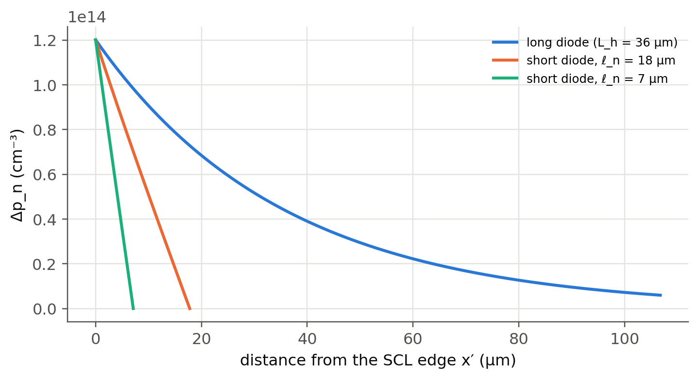
The injected minority carriers diffuse into the neutral region and recombine. In a long neutral region the excess decays
exponentially, $\Delta p_n(x')=\Delta p_n(0)e^{-x'/L_h}$, with **diffusion length** $L_h=\sqrt{D_h\tau_h}$ and Einstein
relation $D=\mu k_BT/e$ (slide 51). The diffusion current gives the **Shockley equation** (slides 52–57):
$$
J=J_{so}\left[\exp\!\left(\frac{eV}{k_BT}\right)-1\right],\qquad J_{so}=\left(\frac{eD_h}{L_hN_d}+\frac{eD_e}{L_eN_a}\right)n_i^2 .
$$
If the neutral region is shorter than $L$ (a **short diode**, slides 59–61), $L_h$ is replaced by its length $\ell_n$.
Carriers also recombine *inside* the SCL, which adds a current with half the exponent (slides 62–65):
$$
J_\text{recom}=J_{ro}\left[\exp\!\left(\frac{eV}{2k_BT}\right)-1\right],\quad J_{ro}=\frac{en_i}{2}\left(\frac{W_p}{\tau_e}+\frac{W_n}{\tau_h}\right),
\qquad J\simeq J_o\left[\exp\!\left(\frac{eV}{\eta k_BT}\right)-1\right].
$$
The **ideality factor** $\eta$ is 1 when diffusion dominates and 2 when SCL recombination dominates. Under reverse bias the
current saturates at the Shockley value plus thermal generation in the SCL (slide 68):
$J_\text{rev}=J_{so}+en_iW/\tau_g$.
## I–V explorer
```{ojs}
//| echo: false
matI = ({
  Si:   {Eg: 1.11, ni: 1.0e10, er: 11.8, mue: 1450, muh: 490, tau: -6},
  Ge:   {Eg: 0.66, ni: 2.3e13, er: 16.0, mue: 3900, muh: 1900, tau: -6},
  GaAs: {Eg: 1.42, ni: 2.1e6,  er: 13.0, mue: 5000, muh: 250, tau: -7.3}
})
viewof iv = Inputs.form({
  mat: Inputs.select(Object.keys(matI), {value: "GaAs", label: "material"}),
  lNa: Inputs.range([15, 19], {value: 17, step: 0.1, label: "log₁₀ N_a (cm⁻³)"}),
  lNd: Inputs.range([15, 19], {value: 17, step: 0.1, label: "log₁₀ N_d (cm⁻³)"}),
  ltau: Inputs.range([-10, -3], {value: -7.3, step: 0.05, label: "log₁₀ lifetime τ (s)"}),
  A: Inputs.range([0.01, 10], {value: 1, step: 0.01, label: "area A (mm²)"})
})
```
```{ojs}
//| echo: false
ivOut = {
  const m = matI[iv.mat], q = 1.602176634e-19, kT = 0.025852, eps = m.er*8.8541878e-12;
  const Na = 10**iv.lNa*1e6, Nd = 10**iv.lNd*1e6, ni = m.ni*1e6, tau = 10**iv.ltau, A = iv.A*1e-6;
  const De = m.mue*1e-4*kT, Dh = m.muh*1e-4*kT, Le = Math.sqrt(De*tau), Lh = Math.sqrt(Dh*tau);
  const Iso = A*q*ni*ni*(Dh/(Lh*Nd) + De/(Le*Na));
  const Vo = kT*Math.log(Na*Nd/ni**2), data = [];
  for (let V = 0.02; V < Vo - 4*kT; V += 0.002) {
    const W = Math.sqrt(2*eps*(Na + Nd)*(Vo - V)/(q*Na*Nd));
    const Iro = A*q*ni/2*W/tau;
    const Id = Iso*Math.expm1(V/kT), Ir = Iro*Math.expm1(V/(2*kT));
    if (Id + Ir > 1) break;
    data.push({V, I: Id + Ir, Id, Ir});
  }
  const eta = data.map((d, i) => i === 0 ? null : {V: d.V, eta: (d.V - data[i-1].V)/(kT*Math.log(d.I/data[i-1].I))}).filter(d => d);
  const cross = data.find(d => d.Id > d.Ir);
  return {data, eta, Iso, Vo, Le, Lh, cross};
}
Plot.plot({
  width: Math.min(width, 1050), height: 340, x: {label: "forward voltage V (V)"},
  y: {type: "log", label: "current (A)", grid: true, domain: [1e-13, 1]},
  color: {legend: true, domain: ["total", "diffusion (η = 1)", "SCL recombination (η = 2)"], range: ["#0b0b0b", "#2a78d6", "#eb6834"]},
  marks: [
    Plot.line(ivOut.data.filter(d => d.Id > 1e-13), {x: "V", y: "Id", stroke: () => "diffusion (η = 1)", strokeWidth: 1.8}),
    Plot.line(ivOut.data.filter(d => d.Ir > 1e-13), {x: "V", y: "Ir", stroke: () => "SCL recombination (η = 2)", strokeWidth: 1.8}),
    Plot.line(ivOut.data.filter(d => d.I > 1e-13), {x: "V", y: "I", stroke: () => "total", strokeWidth: 2.5}),
    Plot.tip(ivOut.data, Plot.pointerX({x: "V", y: "I", title: d => `V = ${d.V.toFixed(3)} V\nI = ${d.I.toExponential(2)} A\ndiffusion fraction ${(100*d.Id/d.I).toFixed(0)} %`}))
  ]
})
```
```{ojs}
//| echo: false
Plot.plot({
  width: Math.min(width, 1050), height: 150, x: {label: "V (V)"}, y: {label: "local η", domain: [0.9, 2.1], grid: true},
  marks: [Plot.line(ivOut.eta, {x: "V", y: "eta", stroke: "#4a3aa7", strokeWidth: 2}), Plot.ruleY([1, 2], {stroke: "#52514e", strokeDasharray: "3,3"})]
})
```
```{ojs}
//| echo: false
html`<div class="result-box">I<sub>so</sub> = ${ivOut.Iso.toExponential(2)} A · V<sub>o</sub> = ${ivOut.Vo.toFixed(3)} V ·
L<sub>e</sub> = ${(ivOut.Le*1e6).toFixed(2)} µm · L<sub>h</sub> = ${(ivOut.Lh*1e6).toFixed(2)} µm ·
diffusion overtakes recombination at <b>V ≈ ${ivOut.cross ? ivOut.cross.V.toFixed(3) + " V" : "never (below 1 A)"}</b></div>`
```
The lower plot is the local ideality factor $\eta=(dV/d\ln I)/(k_BT/e)$, which you measure from the slope of a semilog I–V
curve (slide 66). Increase the lifetime: recombination in the SCL weakens and the crossover moves to lower voltage. Shorter
lifetimes (more defects) do the opposite.
## Worked example: a GaAs pn junction (slides 75–80), recomputed
> Symmetric GaAs junction, $N_a=N_d=10^{17}$ cm⁻³, $B=2\times10^{-16}$ m³ s⁻¹, $A=1$ mm², $\mu_h=250$ and $\mu_e=5000$
> cm² V⁻¹ s⁻¹, $n_i=2.1\times10^6$ cm⁻³, $\varepsilon_r=13$. Find the diffusion and recombination currents at 0.80 V and 1.05 V,
> taking the SCL lifetimes equal to the neutral-region lifetimes $\tau=1/(BN)$.
```{python}
#| label: tbl-gaas-diode
#| tbl-cap: "The GaAs diode of slides 75–80. Slide values: τ = 50 ns, D_h = 6.46×10⁻⁴ and D_e = 1.29×10⁻² m²/s, L_h = 5.69 µm, L_e = 25.4 µm, I_so ≈ 4.4×10⁻²¹ A, V_o = 1.27 V, W = 0.116 µm and I_ro ≈ 3.9×10⁻¹³ A at 0.8 V; I_diff = 0.12 µA and I_recom = 2.0 µA at 0.8 V; 1.9 mA and 0.18 mA at 1.05 V."
gaas = dict(A=1e-6, Na=1e23, Nd=1e23, mat="GaAs", B=2e-16, mu_e=5000*CM2, mu_h=250*CM2)
rows = {}
for V in (0.80, 1.05):
    d = sl.diode_currents(V, **gaas)
    rows[f"V = {V:.2f} V"] = {"τ (ns)": d["tau_h"]*1e9, "D_h (m²/s)": f"{d['Dh']:.3g}", "D_e (m²/s)": f"{d['De']:.3g}",
        "L_h (µm)": d["Lh"]*1e6, "L_e (µm)": d["Le"]*1e6, "I_so (A)": f"{d['Iso']:.2e}", "V_o (V)": d["Vo"],
        "W (µm)": d["W"]*1e6, "I_ro (A)": f"{d['Iro']:.2e}", "I_diff": f"{d['I_diff']:.3g} A", "I_recom": f"{d['I_rec']:.3g} A",
        "η (local)": None}
    dV = 1e-3; d2 = sl.diode_currents(V + dV, **gaas)
    rows[f"V = {V:.2f} V"]["η (local)"] = round(dV/(sl.kT()*np.log(d2["I"]/d["I"])), 2)
pd.DataFrame(rows).round(3)
```
All values agree with the slides. At 0.8 V the recombination current is 17 times the diffusion current ($\eta\approx2$). At 1.05 V diffusion
dominates ($\eta\approx1$). Every recombination event in GaAs can emit a photon of energy $\approx E_g$: this is the LED of
the next chapters.
## Minority carrier profiles: long and short diodes (slides 51, 59–61)
```{python}
#| label: fig-profiles
#| fig-cap: "Excess hole concentration in the neutral n side of a Si diode (N_d = 10¹⁶ cm⁻³, τ_h = 1 µs, V = 0.6 V). Long diode: exponential decay over L_h. Short diodes (ℓ_n < L_h, ohmic contact at ℓ_n where Δp = 0): nearly linear profile, steeper gradient and therefore a larger diffusion current."
Nd, tau_h = 1e16*CM3, 1e-6
ni = sl.MATERIALS["Si"]["ni"]; Dh = sl.einstein_D(sl.MATERIALS["Si"]["mu_h"]); Lh = np.sqrt(Dh*tau_h)
dp0 = ni**2/Nd*np.expm1(0.6/sl.kT())
fig, ax = plt.subplots(figsize=(7.5, 3.6))
x = np.linspace(0, 3*Lh, 400)
ax.plot(x*1e6, dp0*np.exp(-x/Lh)/CM3, label=f"long diode (L_h = {Lh*1e6:.0f} µm)")
for ln in (0.5*Lh, 0.2*Lh):
    xs = np.linspace(0, ln, 200)
    ax.plot(xs*1e6, dp0*np.sinh((ln - xs)/Lh)/np.sinh(ln/Lh)/CM3, label=f"short diode, ℓ_n = {ln*1e6:.0f} µm")
ax.set(xlabel="distance from the SCL edge x′ (µm)", ylabel="Δp_n (cm⁻³)"); ax.legend(fontsize=8); plt.show()
tt = (0.2*Lh)**2/(2*Dh)
print(f"Δp_n(0) = {dp0/CM3:.2e} cm⁻³;  transit time of the 0.2 L_h short diode τ_t = ℓ²/2D = {tt*1e9:.0f} ns  (vs τ_h = {tau_h*1e9:.0f} ns)")
```
The exact profile for any $\ell_n$ is $\Delta p_n(0)\sinh[(\ell_n-x')/L_h]/\sinh(\ell_n/L_h)$, which tends to the long-diode
exponential for $\ell_n\gg L_h$ and to a straight line for $\ell_n\ll L_h$. The short diode "replenishes" its stored charge every
transit time $\tau_t=\ell_n^2/2D_h$ instead of every lifetime: this is why it is faster (@sec-smallsignal).
## Ge, Si and GaAs diodes (slides 58 and 66)
```{python}
#| label: fig-iv-materials
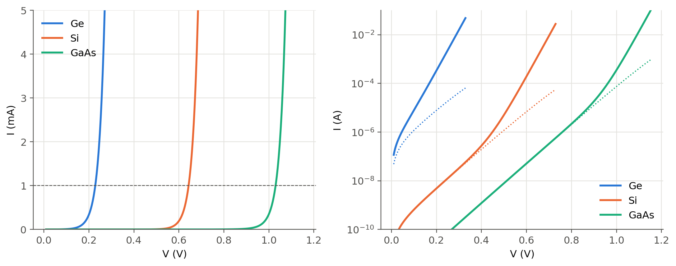
#| fig-cap: "Forward I–V curves of Ge, Si and GaAs junctions (N_a = N_d = 10¹⁷ cm⁻³, A = 1 mm², τ = 1 µs for Ge and Si, 50 ns for GaAs, Table 3.1 mobilities; GaAs uses the slide-75 mobilities). Left: linear scale with the familiar 'turn-on' voltages. Right: log scale (slide 66) with η = 2 at low bias (dotted guide lines) and η = 1 at high bias."
V = np.linspace(0.01, 1.3, 600)
pars = {"Ge": dict(tau_e=1e-6, tau_h=1e-6), "Si": dict(tau_e=1e-6, tau_h=1e-6),
        "GaAs": dict(tau_e=50e-9, tau_h=50e-9, mu_e=5000*CM2, mu_h=250*CM2)}
fig, ax = plt.subplots(1, 2, figsize=(10, 4))
for m, kw in pars.items():
    Vo = sl.built_in_voltage(1e23, 1e23, sl.MATERIALS[m]["ni"])
    Vm = V[V < Vo - 4*sl.kT()]
    d = sl.diode_currents(Vm, 1e-6, 1e23, 1e23, m, **kw)
    ok = d["I"] < 0.1
    ax[0].plot(Vm[ok], d["I"][ok]*1e3, label=m)
    ax[1].semilogy(Vm[ok], d["I"][ok], label=m)
    ax[1].semilogy(Vm[ok], d["I_rec"][ok], ":", color=ax[1].lines[-1].get_color(), lw=1.2)
ax[0].set(xlabel="V (V)", ylabel="I (mA)", ylim=(0, 5)); ax[0].axhline(1, color=sl.INK2, lw=0.8, ls="--"); ax[0].legend()
ax[1].set(xlabel="V (V)", ylabel="I (A)", ylim=(1e-10, 0.1)); ax[1].legend()
plt.tight_layout(); plt.show()
```
The "turn-on" voltage at 1 mA is roughly $E_g/e$ minus a few tenths of a volt. It scales with the bandgap because $J_{so}\propto
n_i^2\propto e^{-E_g/k_BT}$. An LED therefore needs a forward voltage close to $h\nu/e$: about 1.2 V for an infrared GaAs LED
and about 3 V for a blue InGaN LED.
## Series resistance (slide 66, "series resistance limitation")
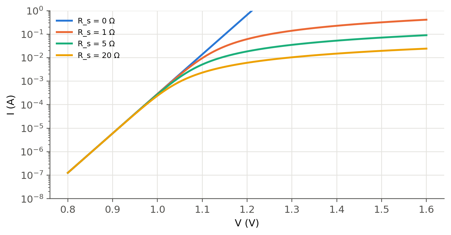
At high current the ohmic drop $IR_s$ in the neutral regions and contacts bends the semilog curve down. The implicit equation
$I=I_o[\exp((V-IR_s)/\eta V_T)-1]$ has an exact solution with the Lambert $W$ function (`sl.diode_iv_rs`):
```{python}
#| label: fig-rs
#| fig-cap: "Effect of the series resistance on a GaAs diode (I_o = 4.6×10⁻²¹ A, η = 1). Above a few mA the voltage drop in R_s dominates, and fitting η there gives meaningless values."
V = np.linspace(0.8, 1.6, 400)
fig, ax = plt.subplots(figsize=(7.5, 3.6))
for Rs in (0, 1, 5, 20):
    ax.semilogy(V, sl.diode_iv_rs(V, 4.6e-21, 1.0, Rs), label=f"R_s = {Rs} Ω")
ax.set(xlabel="V (V)", ylabel="I (A)", ylim=(1e-8, 1)); ax.legend(fontsize=8); plt.show()
```
## Reverse current and temperature (slides 67–69)
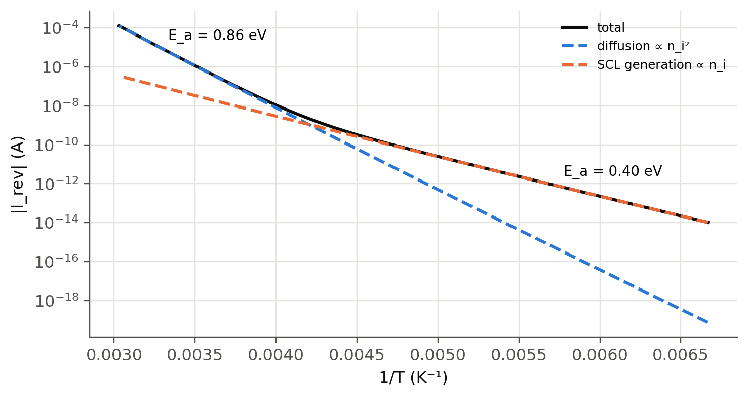
Under reverse bias the diffusion part saturates at $-J_{so}\propto n_i^2$ and the SCL generation part $-en_iW/\tau_g\propto n_i$
grows slowly with $W$. Because $n_i\propto e^{-E_g/2k_BT}$, an Arrhenius plot of $I_\text{rev}$ shows two slopes: $E_g$ at high
temperature (diffusion) and $E_g/2$ at low temperature (generation). Slide 69 measures 0.63 eV and 0.33 eV on a Ge photodiode
with the crossover at 238 K. The code chooses the generation time $\tau_g$ so that the crossover falls at the same temperature:
```{python}
#| label: fig-reverse-T
#| fig-cap: "Reverse current at V = −5 V of a Ge p⁺n diode (N_a = 10¹⁸, N_d = 10¹⁵ cm⁻³, A = 1 mm², τ = 1 µs) against 1/T. The two fitted activation energies differ by a factor of two, as in slide 69."
kw = dict(A=1e-6, Na=1e18*CM3, Nd=1e15*CM3, mat="Ge", tau_e=1e-6, tau_h=1e-6)
def parts(T, tg): d = sl.diode_currents(-5.0, T=T, tau_g=tg, **kw); return -d["I_diff"], -d["I_rec"]
tg = 10**brentq(lambda lt: np.log(parts(238, 10**lt)[0]/parts(238, 10**lt)[1]), -9, 3)
T = np.linspace(150, 330, 60)
Id, Ig = np.array([parts(t, tg) for t in T]).T
fig, ax = plt.subplots(figsize=(7.5, 3.8))
ax.semilogy(1/T, Id + Ig, color=sl.INK, label="total")
ax.semilogy(1/T, Id, "--", label="diffusion ∝ n_i²"); ax.semilogy(1/T, Ig, "--", label="SCL generation ∝ n_i")
for sel, lab in ((T > 270, "hot"), (T < 200, "cold")):
    s = np.polyfit(1/T[sel], np.log((Id + Ig)[sel]), 1)[0]
    ax.text(np.mean(1/T[sel]), np.exp(np.polyval(np.polyfit(1/T[sel], np.log((Id + Ig)[sel]), 1), np.mean(1/T[sel])))*4,
            f"E_a = {-s*sl.kB/sl.qe:.2f} eV", fontsize=9)
ax.set(xlabel="1/T (K⁻¹)", ylabel="|I_rev| (A)"); ax.legend(fontsize=8); plt.show()
print(f"generation time chosen for a 238 K crossover: τ_g = {tg:.2e} s")
```
The model gives about 0.86 eV and 0.40 eV, higher than the slide values, but with the same factor of two. An Arrhenius
slope does not measure $E_g(300 ext{ K})$. It measures the bandgap extrapolated linearly to 0 K (about 0.78 eV for Ge with the
Varshni law) plus about $3k_BT$ (or $1.5k_BT$) from the $T^3$ ($T^{3/2}$) prefactor of $n_i^2$ ($n_i$). The lower slopes
measured on slide 69 point to extra temperature-dependent factors in the real photodiode, such as lifetimes and surface
leakage. Comparing the model with the measurement is a good exercise.
::: {.callout-tip collapse="true"}
## Going deeper
- **High injection.** When $\Delta p_n(0)$ approaches $N_d$, the current goes as $\exp(eV/2k_BT)$ again. Derive it from
neutrality in the n region. Where does it start for the GaAs example?
- **Temperature coefficient of $V_F$.** At constant current, $dV/dT\approx-(E_g/e-V)/T\approx-2$ mV/K for Si. Check it with
`sl.diode_currents` at two temperatures. This is how LED junction temperature is measured (@sec-spectrum).
- **Fit a real diode.** Measure an LED I–V with a source-meter (or use a datasheet curve). Fit $I_o$, $\eta$ and $R_s$ with
`scipy.optimize.curve_fit` and `sl.diode_iv_rs`.
- **Shockley–Read–Hall.** The $\eta=2$ current comes from recombination through mid-gap traps. Integrate the SRH rate
$U=(np-n_i^2)/[\tau(n+p+2n_i)]$ across the SCL numerically and compare with $J_{ro}$.
:::
::: {.callout-note collapse="true"}
## Complements
- Kasap, *Optoelectronics and Photonics*, sec. 3.4–3.6; Sze & Ng, ch. 2.
- C.-T. Sah, R. N. Noyce, W. Shockley, "Carrier generation and recombination in p–n junctions", *Proc. IRE* 45, 1228 (1957).
- D. Scansen and S. O. Kasap, *Can. J. Phys.* 70, 1070 (1992): the Ge reverse-current data of slide 69.
:::
## Try it yourself
1. With the GaAs parameters, at which forward voltage are the diffusion and recombination currents equal?
2. A Si diode has $I_o=10^{-14}$ A, $\eta=1$. Which voltage gives 1 mA? By how much must $V$ rise to get 10 mA?
3. Compute $I_{so}$ of the GaAs example if the p region is only 2 µm long (short diode on the p side, $\ell_p<L_e$).
4. In the explorer, find a set of Si parameters where diffusion dominates already at 0.3 V. What does this require physically?