# Efficiency, brightness and white LEDs {#sec-efficiency}
[](https://colab.research.google.com/github/{{< var github_user >}}/{{< var repo >}}/blob/main/{{< var subdir >}}/notebooks/efficiency.ipynb){.colab-link} Run this chapter's code in Google Colab (no installation).
```{python}
#| include: false
import numpy as np
import matplotlib.pyplot as plt
import pandas as pd
import semilib as sl
sl.use_style()
```
*Slides 120–133 (light extraction, DBR LEDs and RCLEDs, internal, extraction, external and power-conversion efficiencies,
luminous flux, the eye's sensitivity, luminous efficacy, LED characteristics) and 139–143 (white LEDs, phosphors).*
## Key relations
Light generated inside the chip meets the semiconductor–air surface. Rays outside the **escape cone** $\sin\theta_c=n_a/n_s$
are totally reflected (slide 120). For isotropic emission the fraction that escapes through one flat face is (slide 122)
$$
\eta_\text{extraction}\approx\tfrac12(1-\cos\theta_c)\,T,\qquad T\approx\frac{4n_sn_a}{(n_s+n_a)^2}.
$$
The chain from electrons to photons is described by four efficiencies (slides 124–130):
$$
\eta_\text{IQE}=\frac{\tau_r^{-1}}{\tau_r^{-1}+\tau_{nr}^{-1}},\qquad
P_o=\eta_\text{EE}\,\eta_\text{IQE}\,h\nu\,\frac{I}{e},\qquad
\eta_\text{EQE}=\frac{P_o/h\nu}{I/e}=\eta_\text{IQE}\eta_\text{EE},\qquad
\eta_\text{PCE}=\frac{P_o}{IV}\approx\eta_\text{EQE}\frac{E_g}{eV}.
$$
The eye does not see watts. The **luminous flux** weighs the optical power with the photopic sensitivity $V(\lambda)$, which peaks
at 555 nm, and the **luminous efficacy** relates it to the electrical power:
$$
\Phi_v=P_o\times683\ \text{lm W}^{-1}\times V(\lambda),\qquad \eta_\text{LE}=\frac{\Phi_v}{IV}.
$$
## LED efficiency calculator
```{ojs}
//| echo: false
Vtab = [3.9e-5, 1.2e-4, 3.96e-4, 1.21e-3, 4.0e-3, 1.16e-2, 2.3e-2, 3.8e-2, 6.0e-2, 9.098e-2, 0.13902, 0.20802, 0.323, 0.503, 0.71, 0.862, 0.954, 0.99495, 0.995, 0.952, 0.87, 0.757, 0.631, 0.503, 0.381, 0.265, 0.175, 0.107, 0.061, 0.032, 0.017, 8.21e-3, 4.102e-3, 2.091e-3, 1.047e-3, 5.2e-4, 2.49e-4, 1.2e-4, 6.0e-5, 3.0e-5, 1.5e-5]
Vphot = (l) => { if (l < 380 || l > 780) return 0; const i = Math.min(39, Math.floor((l - 380)/10)), f = (l - 380 - 10*i)/10;
  return Math.exp(Math.log(Vtab[i])*(1 - f) + Math.log(Vtab[i + 1])*f); }
viewof ef = Inputs.form({
  lam: Inputs.range([380, 1000], {value: 625, step: 1, label: "emission wavelength λ (nm)"}),
  I: Inputs.range([1, 1000], {value: 350, step: 1, label: "drive current I (mA)"}),
  V: Inputs.range([1, 4.5], {value: 2.2, step: 0.01, label: "forward voltage V (V)"}),
  iqe: Inputs.range([0.05, 1], {value: 0.85, step: 0.01, label: "internal quantum efficiency"}),
  ns: Inputs.range([1.5, 4], {value: 3.3, step: 0.01, label: "chip refractive index n_s"}),
  na: Inputs.range([1, 1.8], {value: 1.5, step: 0.01, label: "encapsulant index n_a (air = 1)"}),
  faces: Inputs.range([1, 6], {value: 1, step: 1, label: "escaping faces (bare cube: up to 6)"})
})
```
```{ojs}
//| echo: false
efOut = {
  const hv = 1239.84/ef.lam, tc = Math.asin(ef.na/ef.ns), T = 4*ef.ns*ef.na/(ef.ns + ef.na)**2;
  const ee = Math.min(1, ef.faces*0.5*(1 - Math.cos(tc))*T);
  const eqe = ef.iqe*ee, Po = eqe*hv*ef.I/1000;            // W
  const pce = Po/(ef.V*ef.I/1000), V = Vphot(ef.lam), phi = 683*Po*V;
  const chain = [{s: "electrical power IV", v: ef.V*ef.I/1000}, {s: "photons generated (IQE)", v: ef.iqe*hv*ef.I/1000},
                 {s: "photons extracted (P_o)", v: Po}];
  return {hv, tc: tc*180/Math.PI, T, ee, eqe, Po, pce, V, phi, le: phi/(ef.V*ef.I/1000), chain};
}
Plot.plot({
  width: Math.min(width, 1050), height: 170, marginLeft: 190, x: {label: "power (W)", grid: true},
  y: {label: null, domain: efOut.chain.map(d => d.s)},
  marks: [Plot.barX(efOut.chain, {y: "s", x: "v", fill: "#2a78d6", rx: 4}),
          Plot.text(efOut.chain, {y: "s", x: "v", text: d => `${(1000*d.v).toFixed(1)} mW`, dx: 6, textAnchor: "start", fill: "#0b0b0b"})]
})
```
```{ojs}
//| echo: false
html`<div class="result-box">hν = ${efOut.hv.toFixed(3)} eV · θ<sub>c</sub> = ${efOut.tc.toFixed(1)}° · T = ${efOut.T.toFixed(3)} ·
extraction η<sub>EE</sub> = <b>${(100*efOut.ee).toFixed(1)} %</b> · EQE = <b>${(100*efOut.eqe).toFixed(1)} %</b><br>
P<sub>o</sub> = <b>${(1000*efOut.Po).toFixed(1)} mW</b> · PCE = ${(100*efOut.pce).toFixed(1)} % · V(λ) = ${efOut.V.toPrecision(3)} ·
Φ<sub>v</sub> = <b>${efOut.phi.toFixed(1)} lm</b> · luminous efficacy = <b>${efOut.le.toFixed(1)} lm/W</b></div>`
```
Extraction is the weak link of a simple chip: even with a perfect IQE, a planar GaAs chip in air emits about 1.5 % per face.
Commercial LEDs reach 60–80 % extraction with shaped chips, textured surfaces, back reflectors, thin-film flip-chip designs and
domes (slides 120–121).
## Worked example: light extraction (slides 122–123), recomputed
> GaAs chip, $n_s=3.4$. Extraction ratio through one face into air ($n_a=1$) and into an epoxy dome with $n_a=1.8$.
```{python}
#| label: tbl-extraction
#| tbl-cap: "Extraction ratio of a planar GaAs chip (one face). The slide gives θc = 17.1°, T = 0.702 and 1.6 % in air; 32° and 6.9 % with epoxy. 'Exact' averages the Fresnel transmittance (unpolarised) over the escape cone instead of using the normal-incidence value."
rows = {}
for na in (1.0, 1.5, 1.8):
    tc = np.degrees(np.arcsin(na/3.4))
    rows[f"n_a = {na}"] = {"θ_c (deg)": round(tc, 1), "T (normal)": round(4*3.4*na/(3.4 + na)**2, 3),
                           "cone fraction ½(1 − cos θc)": f"{0.5*(1 - np.cos(np.radians(tc)))*100:.2f} %",
                           "extraction (slide formula)": f"{sl.extraction_ratio(3.4, na)*100:.2f} %",
                           "extraction (exact Fresnel)": f"{sl.extraction_ratio(3.4, na, exact=True)*100:.2f} %"}
pd.DataFrame(rows).T
```
```{python}
#| label: fig-extraction
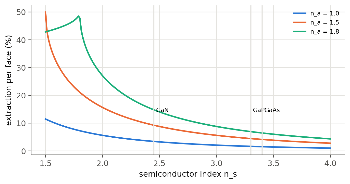
#| fig-cap: "One-face extraction ratio versus the chip index for three ambients. High-index semiconductors trap most of their light; the encapsulant helps by a factor of 3–4. The dome of slide 120(b) removes the second (dome–air) TIR only if it is large and hemispherical."
ns = np.linspace(1.5, 4, 200)
fig, ax = plt.subplots(figsize=(7.5, 3.6))
for na in (1.0, 1.5, 1.8):
    ax.plot(ns, [sl.extraction_ratio(n, na, exact=True)*100 for n in ns], label=f"n_a = {na}")
for name, n in (("GaN", 2.45), ("GaP", 3.3), ("GaAs", 3.4)):
    ax.axvline(n, color=sl.GRID, lw=1.5); ax.text(n + 0.02, 14, name, fontsize=8)
ax.set(xlabel="semiconductor index n_s", ylabel="extraction per face (%)"); ax.legend(fontsize=8); plt.show()
```
## The eye's sensitivity and LED brightness (slides 128–133)
```{python}
#| label: fig-vlambda
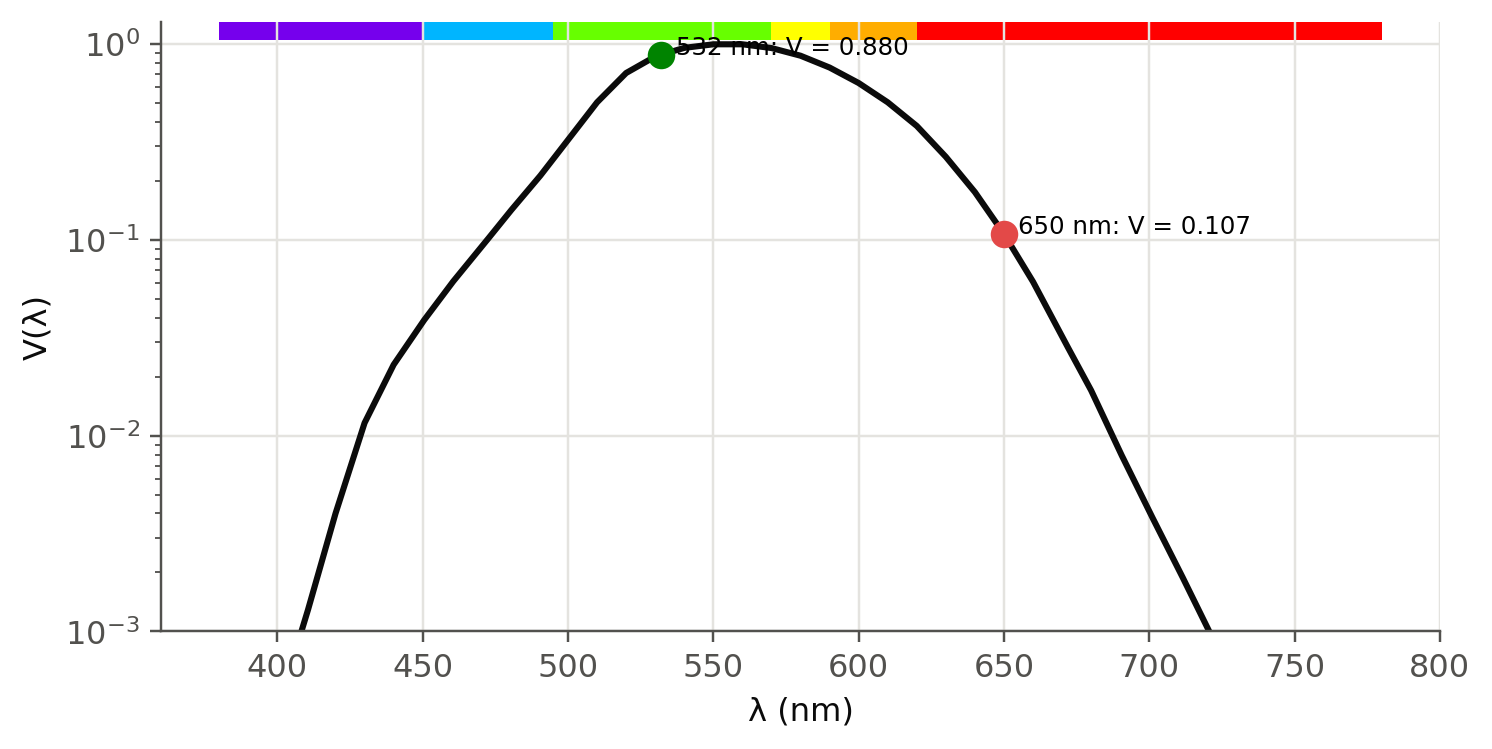
#| fig-cap: "Photopic luminous efficiency V(λ) (CIE 1924) on a logarithmic scale (slide 129), with the two LEDs of slide 133 marked."
lam = np.linspace(380, 780, 801)
fig, ax = plt.subplots(figsize=(7.5, 3.6))
for lo, hi in ((380, 450), (450, 495), (495, 570), (570, 590), (590, 620), (620, 780)):
    ax.axvspan(lo, hi, ymin=0.97, ymax=1, color=sl.wavelength_rgb((lo + hi)/2), lw=0)
ax.semilogy(lam, sl.V_photopic(lam*1e-9), color=sl.INK)
for l, c in ((650, sl.PALETTE[7]), (532, sl.PALETTE[5])):
    ax.plot(l, sl.V_photopic(l*1e-9), "o", ms=8, color=c); ax.text(l + 5, sl.V_photopic(l*1e-9), f"{l} nm: V = {float(sl.V_photopic(l*1e-9)):.3f}", fontsize=8)
ax.set(xlabel="λ (nm)", ylabel="V(λ)", ylim=(1e-3, 1.3)); plt.show()
```
> **Slide 133.** A 10 mW red LED at 650 nm and a 5 mW green LED at 532 nm. Find the luminous flux of each.
```{python}
#| label: tbl-brightness
#| tbl-cap: "Slide 133 recomputed. The slide reads V ≈ 0.10 and 0.87 from the graph and obtains 0.68 lm and 3.0 lm."
pd.DataFrame({f"{P*1e3:.0f} mW at {l} nm": {"V(λ) (CIE table)": round(float(sl.V_photopic(l*1e-9)), 3),
                                            "Φv (lm)": round(float(sl.luminous_flux(P, l*1e-9)), 2),
                                            "Φv with the slide's V": round(683*P*v, 2)}
              for P, l, v in ((10e-3, 650, 0.10), (5e-3, 532, 0.87))}).T
```
The green LED is four times brighter with half the power. Note a typo on slide 133: the equation is written with
"633 lm W⁻¹", but the numbers use the correct 683 lm W⁻¹.
## White LEDs (slides 139–143)
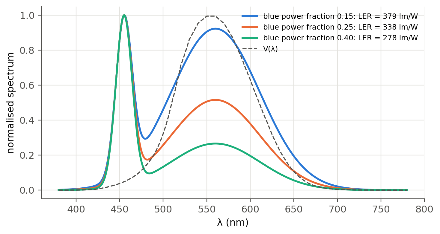
A blue InGaN chip excites a Ce:YAG phosphor. Part of the blue light passes through and the phosphor converts the rest into broad
yellow emission. Together they look white. Each converted photon loses the energy difference between blue and yellow (the
**Stokes loss**). The **luminous efficacy of radiation** (LER, lumens per optical watt) depends only on the spectrum:
```{python}
#| label: fig-white
#| fig-cap: "Model white-LED spectra: blue InGaN line (455 nm, 22 nm FWHM) plus Ce:YAG phosphor band (560 nm, 120 nm FWHM) for three blue fractions, with V(λ) dashed. Less blue gives higher LER but a yellowish, 'warmer' colour; the phosphor's Stokes loss limits the overall efficiency."
lam = np.linspace(380, 780, 2001)*1e-9
gauss = lambda l0, fw: np.exp(-4*np.log(2)*((lam - l0)/fw)**2)
blue, yag = gauss(455e-9, 22e-9), gauss(560e-9, 120e-9)
fig, ax = plt.subplots(figsize=(7.5, 3.8))
rows = {}
for fb in (0.15, 0.25, 0.40):
    S = fb*blue/np.trapezoid(blue, lam) + (1 - fb)*yag/np.trapezoid(yag, lam)
    LER = sl.luminous_flux(1.0, spectrum=(lam, S))
    ax.plot(lam*1e9, S/S.max(), label=f"blue power fraction {fb:.2f}: LER = {LER:.0f} lm/W")
    stokes = (1 - fb)*(1 - 455/560)                       # fraction of optical power lost in conversion
    rows[f"{fb:.2f}"] = {"LER (lm/W_opt)": round(LER), "Stokes loss (% of blue pump)": round(100*(1 - 455/560)),
                         "efficacy if PCE(blue) = 60 % (lm/W_el)": round(LER*0.60*(1 - stokes))}
ax.plot(lam*1e9, sl.V_photopic(lam), "--", color=sl.INK2, lw=1.2, label="V(λ)")
ax.set(xlabel="λ (nm)", ylabel="normalised spectrum"); ax.legend(fontsize=8); plt.show()
pd.DataFrame(rows).T.rename_axis("blue fraction")
```
The last column is a rough estimate. It assumes the blue chip converts 60 % of the electrical power into blue light and neglects
phosphor quantum-efficiency and package losses. The result, 150–200 lm/W, is close to today's best commercial white LEDs.
Incandescent lamps give about 15 lm/W and fluorescent tubes 60–100 lm/W (slide 131).
```{python}
#| eval: false
# With the optional colour-science package you can compute the chromaticity and the colour temperature (CCT):
import colour
sd = colour.SpectralDistribution(dict(zip(np.round(lam*1e9).astype(int), S)))
XYZ = colour.sd_to_XYZ(sd); xy = colour.XYZ_to_xy(XYZ)
print("chromaticity", xy, "CCT", colour.xy_to_CCT(xy, method="McCamy 1992"), "K")
```
::: {.callout-tip collapse="true"}
## Going deeper
- **Photon recycling.** Light that is totally reflected can be reabsorbed and re-emitted. With an IQE near 1, a chip can therefore
extract much more than the single-pass escape cone. Write a Monte Carlo ray tracer for a cube with absorption and recycling.
- **Efficiency droop.** The ABC model $I/(eV_\text{act})=An+Bn^2+Cn^3$ gives $\eta_\text{IQE}=Bn^2/(An+Bn^2+Cn^3)$. Fit $A$, $B$, $C$ to
a measured EQE–current curve of a blue LED and find the current of peak efficiency.
- **Resonant-cavity LED** (slide 121e). Put the active layer in a Fabry–Perot cavity formed by two DBRs (Chapter 1). Compute the
enhancement of the emission along the normal and the narrowing of the spectrum with the transfer-matrix code `optolib.tmm`.
- **Colour rendering.** Compute the CRI of the model white LED with `colour-science`. Why do "full-spectrum" LEDs use several
phosphors (or violet pumps)?
:::
::: {.callout-note collapse="true"}
## Complements
- Kasap, *Optoelectronics and Photonics*, sec. 3.13–3.15; Schubert, *Light-Emitting Diodes*, ch. 9–10 (extraction), 16–21 (photometry, white LEDs).
- CIE photometric data tables (CIE 018:2019).
- J. Cho *et al.*, "White light-emitting diodes: History, progress, and future", *Laser Photonics Rev.* 11, 1600147 (2017).
:::
## Try it yourself
1. An AlGaInP LED at 625 nm emits 300 mW at 700 mA and 2.3 V. Compute EQE, PCE, Φv and the luminous efficacy.
2. A GaN chip ($n_s=2.45$) is encapsulated in silicone ($n_a=1.5$). What is its one-face extraction ratio? And for all six faces?
3. At equal optical power, which is brighter: a 590 nm amber LED or a 470 nm blue LED? By how much?
4. Find the blue fraction that maximises the LER of the model white LED. Why is that spectrum not used in practice?