# Carrier statistics {#sec-stats}
[](https://colab.research.google.com/github/{{< var github_user >}}/{{< var repo >}}/blob/main/{{< var subdir >}}/notebooks/statistics.ipynb){.colab-link} Run this chapter's code in Google Colab (no installation).
```{python}
#| include: false
import numpy as np
import matplotlib.pyplot as plt
import pandas as pd
import semilib as sl
sl.use_style()
CM3 = sl.CM3
```
*Slides 10–17 and 25: electron and hole concentrations, effective density of states, mass action law, intrinsic Fermi
level, average electron energy, the meaning of $E_F$, Table 3.1.*
## Key relations
The electron concentration in the CB is the area under $g_{cb}(E)f(E)$ (slide 10). When $E_c-E_F\gg k_BT$ (a
**non-degenerate** semiconductor) the Fermi–Dirac function reduces to a Boltzmann tail and the integral is analytic (slides
11–13):
$$
n=N_c\exp\!\left[-\frac{E_c-E_F}{k_BT}\right],\qquad p=N_v\exp\!\left[-\frac{E_F-E_v}{k_BT}\right],\qquad
N_{c,v}=2\left(\frac{2\pi m_{e,h}^*k_BT}{h^2}\right)^{3/2}.
$$
Their product does not depend on $E_F$. This is the **mass action law** (slide 14), valid in equilibrium and in the dark:
$$
np=n_i^2=N_cN_v\exp\!\left(-\frac{E_g}{k_BT}\right).
$$
In an intrinsic semiconductor $n=p=n_i$, which places the Fermi level slightly off mid-gap (slide 15):
$E_{Fi}=E_v+\tfrac12E_g-\tfrac12k_BT\ln(N_c/N_v)=E_v+\tfrac12E_g-\tfrac34k_BT\ln(m_e^*/m_h^*)$. Electrons in the CB have an
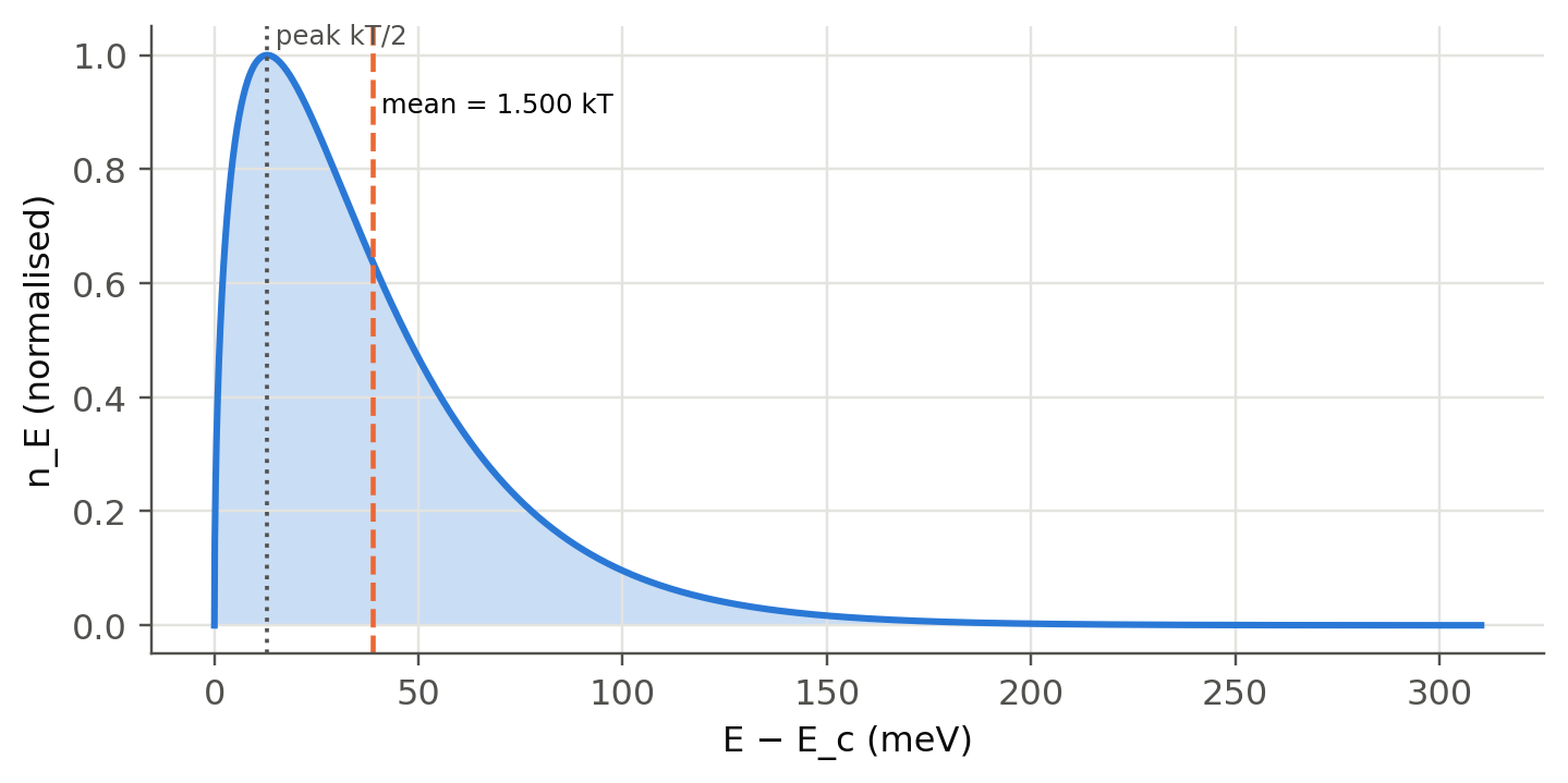
average energy $E_c+\tfrac32k_BT$ above the band edge, like the atoms of an ideal gas (slide 16).
## Electrons and holes in the bands, live
Choose a material, a temperature and a Fermi-level position. The panel integrates $g(E)f(E)$ numerically (no Boltzmann
approximation) and compares the result with the formulas above. Move $E_F$ inside a band to see the Boltzmann formula fail:
that is a **degenerate** semiconductor (@sec-degenerate).
```{ojs}
//| echo: false
mats = ({
  Ge:   {Eg: 0.66, Nc: 1.04e19, Nv: 6.0e18},
  Si:   {Eg: 1.11, Nc: 2.8e19,  Nv: 1.2e19},
  InP:  {Eg: 1.35, Nc: 5.2e17,  Nv: 1.1e19},
  GaAs: {Eg: 1.42, Nc: 4.7e17,  Nv: 7.0e18}
})
viewof st = Inputs.form({
  mat: Inputs.select(Object.keys(mats), {value: "Si", label: "material"}),
  T: Inputs.range([50, 600], {value: 300, step: 5, label: "temperature T (K)"}),
  fe: Inputs.range([-0.15, 1.15], {value: 0.75, step: 0.005, label: "(E_F − E_v)/E_g"})
})
```
```{ojs}
//| echo: false
stOut = {
  const m = mats[st.mat], kT = 8.617333e-5*st.T, Eg = m.Eg, EF = st.fe*Eg;
  const Nc = m.Nc*(st.T/300)**1.5, Nv = m.Nv*(st.T/300)**1.5;
  // DOS normalised so that the Boltzmann integral gives Nc: g = Nc * 2/sqrt(pi) * sqrt(x)/kT
  const f = (E) => 1/(1 + Math.exp((E - EF)/kT)), fh = (E) => 1/(1 + Math.exp((EF - E)/kT));  // fh = 1 − f without cancellation
  const cb = [], vb = []; let n = 0, p = 0; const dE = kT/200;
  for (let x = dE/2; x < 40*kT + Math.max(0, EF - Eg) + Math.max(0, -EF); x += dE) {   // midpoint rule
    const gc = Nc*2/Math.sqrt(Math.PI)*Math.sqrt(x/kT)/kT, gv = Nv*2/Math.sqrt(Math.PI)*Math.sqrt(x/kT)/kT;
    const ne = gc*f(Eg + x), pe = gv*fh(-x);
    n += ne*dE; p += pe*dE;
    cb.push({E: Eg + x, d: ne}); vb.push({E: -x, d: pe});
  }
  const ni = Math.sqrt(Nc*Nv)*Math.exp(-Eg/(2*kT));
  const nB = Nc*Math.exp(-(Eg - EF)/kT), pB = Nv*Math.exp(-EF/kT);
  const EFi = Eg/2 - 0.5*kT*Math.log(Nc/Nv);
  const peak = Math.max(...cb.map(d => d.d), ...vb.map(d => d.d));
  return {cb: cb.filter(d => d.E < Eg + 12*kT + Math.max(0, EF - Eg)), vb: vb.filter(d => d.E > -12*kT - Math.max(0, -EF)),
          n, p, ni, nB, pB, EF, EFi, Eg, peak, kT};
}
Plot.plot({
  width: Math.min(width, 1050), height: 380,
  x: {label: "carriers per unit energy (cm⁻³ eV⁻¹, each band scaled to its own maximum)", domain: [0, 1.05]},
  y: {label: "E − E_v (eV)", grid: true},
  marks: [
    Plot.areaX(stOut.cb, {y: "E", x: d => d.d/Math.max(...stOut.cb.map(e => e.d)), fill: "#2a78d6", fillOpacity: 0.35}),
    Plot.lineX(stOut.cb, {y: "E", x: d => d.d/Math.max(...stOut.cb.map(e => e.d)), stroke: "#2a78d6", strokeWidth: 2}),
    Plot.areaX(stOut.vb, {y: "E", x: d => d.d/Math.max(...stOut.vb.map(e => e.d)), fill: "#eb6834", fillOpacity: 0.35}),
    Plot.lineX(stOut.vb, {y: "E", x: d => d.d/Math.max(...stOut.vb.map(e => e.d)), stroke: "#eb6834", strokeWidth: 2}),
    Plot.ruleY([0, stOut.Eg], {stroke: "#0b0b0b", strokeWidth: 1.5}),
    Plot.ruleY([stOut.EF], {stroke: "#4a3aa7", strokeWidth: 2, strokeDasharray: "6,4"}),
    Plot.ruleY([stOut.EFi], {stroke: "#52514e", strokeWidth: 1, strokeDasharray: "2,3"}),
    Plot.text([{y: stOut.EF, t: "E_F"}, {y: stOut.EFi, t: "E_Fi"}, {y: stOut.Eg, t: "E_c"}, {y: 0, t: "E_v"}],
              {x: 1.03, y: "y", text: "t", textAnchor: "end", dy: -6, fill: "#52514e"})
  ]
})
```
```{ojs}
//| echo: false
html`<div class="result-box">n = <b>${stOut.n.toExponential(2)}</b> cm⁻³ (Boltzmann formula: ${stOut.nB.toExponential(2)}) ·
p = <b>${stOut.p.toExponential(2)}</b> cm⁻³ (Boltzmann: ${stOut.pB.toExponential(2)})<br>
n<sub>i</sub> = ${stOut.ni.toExponential(2)} cm⁻³ · np/n<sub>i</sub>² = ${(stOut.n*stOut.p/stOut.ni**2).toFixed(3)} ·
E<sub>Fi</sub> − E<sub>v</sub> = ${stOut.EFi.toFixed(3)} eV · k<sub>B</sub>T = ${(1000*stOut.kT).toFixed(1)} meV
${Math.min(stOut.Eg - stOut.EF, stOut.EF) < 3*stOut.kT ? html`<br><b>E<sub>F</sub> is within 3k<sub>B</sub>T of a band edge: degenerate, the Boltzmann formulas fail.</b>` : ""}</div>`
```
## Table 3.1 and the effective masses {#sec-table31}
```{python}
#| label: tbl-31
#| tbl-cap: "Table 3.1 of the slides (300 K), with n_i recomputed from √(NcNv) exp(−Eg/2kT) and the density-of-states effective masses implied by Nc and Nv."
rows = {}
for m, p in sl.MATERIALS.items():
    mass = lambda N: (N/2)**(2/3)*sl.h**2/(2*np.pi*sl.kB*300)/sl.me
    rows[m] = {"a (nm)": p["a"]*1e9, "Eg (eV)": p["Eg"], "χ (eV)": p["chi"],
               "Nc (cm⁻³)": f"{p['Nc']/CM3:.2e}", "Nv (cm⁻³)": f"{p['Nv']/CM3:.2e}",
               "ni table (cm⁻³)": f"{p['ni']/CM3:.1e}",
               "ni = √(NcNv)e^(−Eg/2kT)": f"{np.sqrt(p['Nc']*p['Nv'])*np.exp(-p['Eg']/(2*sl.kT()))/CM3:.1e}",
               "ε_r": p["eps_r"], "μe (cm²/Vs)": p["mu_e"]/sl.CM2, "μh (cm²/Vs)": p["mu_h"]/sl.CM2,
               "me*/me": round(mass(p["Nc"]), 3), "mh*/me": round(mass(p["Nv"]), 3)}
pd.DataFrame(rows).T
```
The recomputed $n_i$ agrees with the table to within the uncertainty of the data (the slide notes that $n_i$ of Si varies
between books; $9.7\times10^9$ cm$^{-3}$ is the modern value). One correction: the slide prints $N_v=6.0\times10^{19}$
cm$^{-3}$ for Ge, but the textbook and the mass action law both require $6.0\times10^{18}$ cm$^{-3}$, which is used here.
## Average energy and the Boltzmann tail (slide 16)
```{python}
#| label: fig-avg
#| fig-cap: "Electron distribution n_E(E) in the CB of a non-degenerate semiconductor at 300 K. It peaks at E_c + kT/2 and its mean is E_c + 3kT/2, the kinetic energy of an ideal-gas atom."
kT = sl.kT(300)
E = np.linspace(0, 12*kT, 3000)
nE = np.sqrt(E)*np.exp(-E/kT)                       # g(E) f(E) up to a constant
mean = np.trapezoid(E*nE, E)/np.trapezoid(nE, E)
fig, ax = plt.subplots(figsize=(7.5, 3.4))
ax.fill_between(E*1e3, nE/nE.max(), alpha=0.25, lw=0); ax.plot(E*1e3, nE/nE.max())
ax.axvline(kT/2*1e3, color=sl.INK2, ls=":", lw=1.2); ax.axvline(mean*1e3, color=sl.PALETTE[1], ls="--", lw=1.5)
ax.text(kT/2*1e3, 1.02, " peak kT/2", fontsize=8, color=sl.INK2); ax.text(mean*1e3, 0.9, f" mean = {mean/kT:.3f} kT", fontsize=8)
ax.set(xlabel="E − E_c (meV)", ylabel="n_E (normalised)"); plt.show()
```
## Intrinsic concentration and temperature
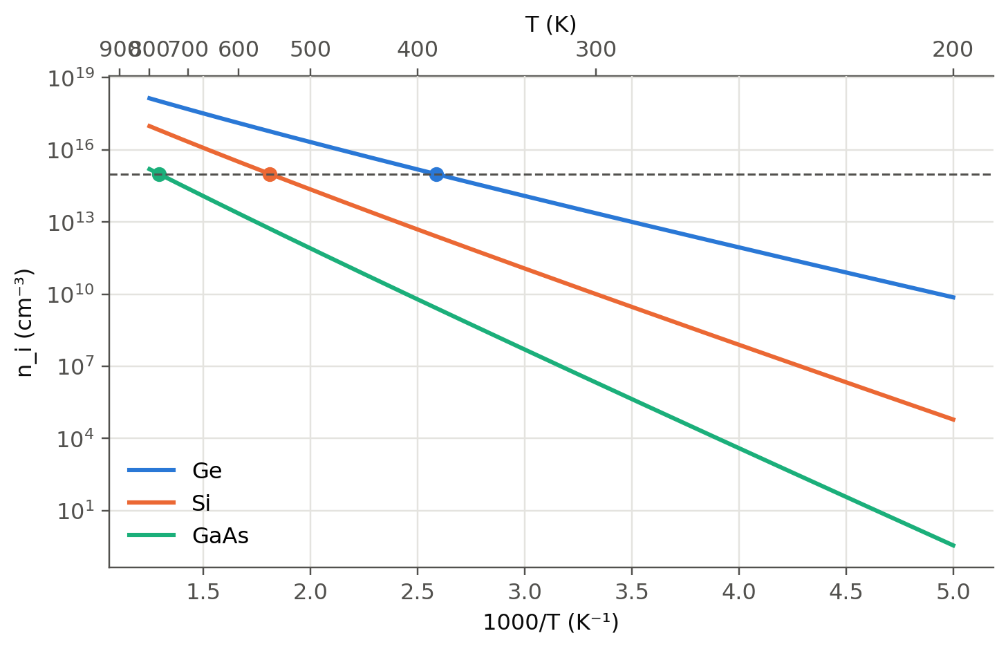
$n_i\propto T^{3/2}\exp(-E_g/2k_BT)$. The exponential dominates, so $\ln n_i$ against $1/T$ is nearly a straight line with
slope $-E_g/2k_B$. The bandgap itself shrinks as $T$ rises (Varshni law, @sec-spectrum), which is included below.
```{python}
#| label: fig-ni
#| fig-cap: "Intrinsic carrier concentration of Ge, Si and GaAs against 1000/T (Nc, Nv ∝ T^{3/2}, Varshni bandgap). The horizontal line is a typical doping of 10¹⁵ cm⁻³: above the crossing temperature the material becomes intrinsic again."
T = np.linspace(200, 800, 400)
fig, ax = plt.subplots()
for m in ("Ge", "Si", "GaAs"):
    ni = sl.n_i(m, T)/CM3
    ax.semilogy(1000/T, ni, label=m)
    Tx = T[np.argmin(abs(np.log(ni/1e15)))]
    if ni.max() > 1e15: ax.plot(1000/Tx, 1e15, "o", color=ax.lines[-1].get_color(), ms=6)
ax.axhline(1e15, color=sl.INK2, ls="--", lw=1)
sec = ax.secondary_xaxis("top", functions=(lambda x: 1000/x, lambda T: 1000/T)); sec.set_xlabel("T (K)")
ax.set(xlabel="1000/T (K⁻¹)", ylabel="n_i (cm⁻³)"); ax.legend(); plt.show()
```
```{python}
#| label: tbl-ni
#| tbl-cap: "Intrinsic concentration and intrinsic Fermi level E_Fi − (E_v + E_g/2) at three temperatures."
out = {}
for m in ("Ge", "Si", "GaAs"):
    p = sl.MATERIALS[m]
    for T in (250, 300, 400):
        Nc, Nv = p["Nc"]*(T/300)**1.5, p["Nv"]*(T/300)**1.5
        out[(m, T)] = {"n_i (cm⁻³)": f"{sl.n_i(m, T)/CM3:.2e}",
                       "E_Fi − midgap (meV)": round(-0.5*sl.kT(T)*np.log(Nc/Nv)*1e3, 1)}
pd.DataFrame(out).T
```
In GaAs the light electron mass ($N_c\ll N_v$) pushes $E_{Fi}$ about 40 meV *above* mid-gap at room temperature.
## When Boltzmann fails {#sec-degenerate}
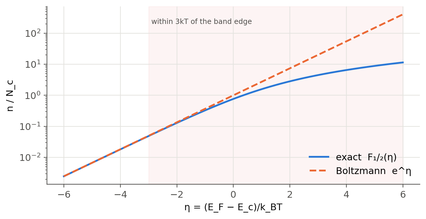
The exact result is $n=N_c\,\mathcal F_{1/2}(\eta)$ with $\eta=(E_F-E_c)/k_BT$ and the Fermi–Dirac integral
$\mathcal F_{1/2}$. The Boltzmann formula is the limit $\mathcal F_{1/2}(\eta)\to e^\eta$:
```{python}
#| label: fig-fermi-int
#| fig-cap: "Exact Fermi–Dirac integral versus the Boltzmann approximation. The error is about 10 % at η ≈ −1 (E_F one kT below E_c) and explodes when E_F enters the band (degenerate semiconductor, slide 28)."
eta = np.linspace(-6, 6, 241)
F = sl.fermi_half(eta)
fig, ax = plt.subplots(figsize=(7.5, 3.6))
ax.semilogy(eta, F, label="exact  F₁/₂(η)"); ax.semilogy(eta, np.exp(eta), "--", label="Boltzmann  e^η")
ax.axvspan(-3, 6, color=sl.PALETTE[7], alpha=0.06); ax.text(-2.9, 200, "within 3kT of the band edge", fontsize=8, color=sl.INK2)
ax.set(xlabel="η = (E_F − E_c)/k_BT", ylabel="n / N_c"); ax.legend(); plt.show()
print("error of Boltzmann at η = -3, -1, 0, +2:", [f"{(np.exp(e)/sl.fermi_half(e) - 1)*100:.0f} %" for e in (-3, -1, 0, 2)])
```
## What the Fermi level means (slide 17)
$E_F$ is the electrochemical potential of electrons. In equilibrium, in the dark and without applied voltage, it is **flat**
across any system of materials in contact. An applied voltage $V$ separates the Fermi levels at the two ends by $\Delta
E_F=eV$. This single rule builds every band diagram in the following chapters: pn junctions (@sec-junction),
heterojunctions (@sec-led), and the quasi-Fermi levels of a forward-biased LED.
::: {.callout-tip collapse="true"}
## Going deeper
- **Density-of-states masses.** Si has six ellipsoidal CB valleys with $m_l=0.98$, $m_t=0.19$. Show that
$m^*_\text{dos}=6^{2/3}(m_lm_t^2)^{1/3}=1.08\,m_e$ and recover $N_c$ of Table 3.1.
- **Joyce–Dixon.** Invert $n=N_c\mathcal F_{1/2}(\eta)$ to get $E_F$ for a given $n$. Compare the Joyce–Dixon series with a
numerical root (`scipy.optimize.brentq` on `sl.fermi_half`).
- **Arrhenius plots.** Fit $\ln(n_iT^{-3/2})$ vs $1/T$ for Si between 250 and 500 K. Which bandgap do you get, and why does
it differ from $E_g(300\text{ K})$? (Hint: Varshni with a linear $T$ term.)
- **Two-dimensional and one-dimensional DOS.** Repeat the counting of slide 4 in 2D and 1D: you get a constant and a
$1/\sqrt{E}$ density of states. The 2D case is the quantum well (@sec-qw).
:::
::: {.callout-note collapse="true"}
## Complements
- Kasap, *Optoelectronics and Photonics*, sec. 3.1–3.2.
- S. M. Sze and K. K. Ng, *Physics of Semiconductor Devices*, ch. 1 (carrier statistics, $\mathcal F_{1/2}$ approximations).
- Ioffe Institute semiconductor database, <https://www.ioffe.ru/SVA/NSM/Semicond/> (band parameters, $n_i(T)$).
:::
## Try it yourself
1. With the live panel, find the temperature at which intrinsic Ge has $n_i=10^{15}$ cm$^{-3}$. Check with the figure.
2. Compute $N_c$ for GaAs from $m_e^*=0.067m_e$ and compare with Table 3.1.
3. Show that $\frac{d\ln n_i}{d(1/T)}=-\frac{E_g}{2k_B}-\frac32T$ and estimate how much the $T^{3/2}$ factor biases a
graphical $E_g$ from 300 to 400 K.
4. Where is $E_{Fi}$ in InP? Is the shift from mid-gap larger or smaller than $k_BT$?