# The LED emission spectrum {#sec-spectrum}
[](https://colab.research.google.com/github/{{< var github_user >}}/{{< var repo >}}/blob/main/{{< var subdir >}}/notebooks/spectrum.ipynb){.colab-link} Run this chapter's code in Google Colab (no installation).
```{python}
#| include: false
import numpy as np
import matplotlib.pyplot as plt
import pandas as pd
import semilib as sl
sl.use_style()
```
*Slides 98–109: energy distribution of carriers, emission spectrum, temperature dependence, worked examples on the
linewidth and on the Varshni shift, degenerately doped junctions.*
## Key relations
Electrons in the CB are spread over a few $k_BT$ above $E_c$, holes a few $k_BT$ below $E_v$ (slide 99). The photon energy is
$h\nu=E_g+(\text{electron KE})+(\text{hole KE})$, so the spectrum follows the joint density of states times the Boltzmann tail:
$$
I(h\nu)\propto(h\nu-E_g)^{1/2}\exp\!\left[-\frac{h\nu-E_g}{k_BT}\right],
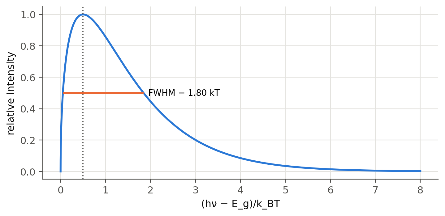
\qquad h\nu_\text{peak}=E_g+\tfrac12k_BT,\qquad \Delta(h\nu)\approx1.8\,k_BT\text{ to }3\,k_BT .
$$
Converting the energy width to wavelength with $|d\lambda/d(h\nu)|=\lambda^2/hc$ gives the **LED linewidth** (slides
103–104):
$$
\Delta\lambda\approx\lambda_o^2\,\frac{3k_BT}{hc}.
$$
The bandgap shrinks with temperature (Varshni law, slide 107): $E_g(T)=E_{go}-AT^2/(B+T)$. The peak moves to longer
wavelengths and the line broadens as the LED warms up.
## Spectrum explorer
```{ojs}
//| echo: false
vars = ({
  "GaAs (870 nm)":          {Eg0: 1.519, A: 5.41e-4, B: 204, off: 0},
  "Al0.06Ga0.94As (≈ 822 nm, slide 101)": {Eg0: 1.519, A: 5.41e-4, B: 204, off: 0.072},
  "InP (≈ 920 nm)":         {Eg0: 1.421, A: 4.9e-4, B: 327, off: 0},
  "InGaAsP (≈ 1310 nm)":    {Eg0: 1.421, A: 4.9e-4, B: 327, off: -0.40},
  "InGaAsP (≈ 1550 nm)":    {Eg0: 1.421, A: 4.9e-4, B: 327, off: -0.545}
})
viewof sp = Inputs.form({
  mat: Inputs.select(Object.keys(vars), {value: "GaAs (870 nm)", label: "active material"}),
  TC: Inputs.range([-60, 150], {value: 25, step: 1, label: "junction temperature (°C)"}),
  sig: Inputs.range([0, 40], {value: 0, step: 1, label: "extra (alloy/inhomogeneous) broadening σ (meV)"})
})
```
```{ojs}
//| echo: false
spOut = {
  const v = vars[sp.mat];
  const curve = (TC, sig) => {
    const T = TC + 273.15, kT = 8.617333e-5*T, Eg = v.Eg0 - v.A*T*T/(v.B + T) + v.off;
    const E = [], I = [];
    for (let i = 0; i <= 500; i++) { const e = Eg - 0.08 + (12*kT + 0.16)*i/500; E.push(e);
      const x = (e - Eg)/kT; I.push(x > 0 ? Math.sqrt(x)*Math.exp(-x) : 0); }
    let J = I;
    if (sig > 0) { const s = sig/1000; J = E.map((e, i) => { let acc = 0, w = 0;
      for (let j = 0; j < E.length; j++) { const g = Math.exp(-((E[j] - e)**2)/(2*s*s)); acc += g*I[j]; w += g; } return acc/w; }); }
    const pts = E.map((e, i) => ({lam: 1239.84/e, I: J[i]}));
    // FWHM in wavelength
    const mx = Math.max(...J), half = pts.filter(d => d.I >= mx/2);
    const lams = half.map(d => d.lam), peak = pts[J.indexOf(mx)].lam;
    return {pts, mx, peak, fwhm: Math.max(...lams) - Math.min(...lams), Eg, kT};
  };
  const ref = curve(25, sp.sig), now = curve(sp.TC, sp.sig);
  const norm = ref.mx;
  return {ref: ref.pts.map(d => ({...d, I: d.I/norm, T: "25 °C"})), now: now.pts.map(d => ({...d, I: d.I/norm, T: `${sp.TC} °C`})),
          peak: now.peak, fwhm: now.fwhm, Eg: now.Eg, kT: now.kT, dpeak: now.peak - ref.peak};
}
Plot.plot({
  width: Math.min(width, 1050), height: 320, x: {label: "λ (nm)"}, y: {label: "relative intensity (25 °C peak = 1)", grid: true},
  marks: [
    Plot.line(spOut.ref, {x: "lam", y: "I", stroke: "#52514e", strokeWidth: 1.4, strokeDasharray: "5,4"}),
    Plot.areaY(spOut.now, {x: "lam", y: "I", fill: "#2a78d6", fillOpacity: 0.2}),
    Plot.line(spOut.now, {x: "lam", y: "I", stroke: "#2a78d6", strokeWidth: 2.2}),
    Plot.tip(spOut.now, Plot.pointerX({x: "lam", y: "I", title: d => `λ = ${d.lam.toFixed(1)} nm\nI = ${d.I.toFixed(3)}`}))
  ]
})
```
```{ojs}
//| echo: false
html`<div class="result-box">E<sub>g</sub>(T) = ${spOut.Eg.toFixed(4)} eV · peak λ<sub>o</sub> = <b>${spOut.peak.toFixed(1)} nm</b>
(${spOut.dpeak >= 0 ? "+" : ""}${spOut.dpeak.toFixed(1)} nm vs 25 °C) · FWHM = <b>${spOut.fwhm.toFixed(1)} nm</b> ·
3k<sub>B</sub>T estimate λ<sub>o</sub>²·3kT/hc = ${(spOut.peak**2*3*spOut.kT/1239.84).toFixed(1)} nm</div>`
```
Dashed: the same LED at 25 °C. Without extra broadening the ideal spectrum has a FWHM of $1.8k_BT$, narrower than the
$3k_BT$ rule of the slides. Real LEDs are broader because of alloy fluctuations, band tails and heating. Add 10–20 meV of
broadening to reach the measured widths.
## The ideal spectrum: peak and width
```{python}
#| label: fig-ideal
#| fig-cap: "Ideal LED spectrum in reduced units x = (hν − E_g)/k_BT. Peak at x = 1/2, half-intensity points at x = 0.05 and 1.85, so FWHM = 1.80 k_BT (slide 99)."
x = np.linspace(0, 8, 80001)
I = np.sqrt(x)*np.exp(-x)
xp = x[np.argmax(I)]; above = x[I >= I.max()/2]
fig, ax = plt.subplots(figsize=(7.5, 3.3))
ax.plot(x, I/I.max()); ax.axvline(xp, ls=":", color=sl.INK2, lw=1.2)
ax.hlines(0.5, above[0], above[-1], color=sl.PALETTE[1], lw=2); ax.text(above[-1] + 0.1, 0.5, f"FWHM = {above[-1] - above[0]:.2f} kT", va="center", fontsize=9)
ax.set(xlabel="(hν − E_g)/k_BT", ylabel="relative intensity"); plt.show()
print(f"peak at {xp:.3f} kT, half-maximum points {above[0]:.3f} and {above[-1]:.3f} kT, FWHM {above[-1] - above[0]:.3f} kT")
```
## Worked examples (slides 103–108), recomputed
> **Slides 103–104.** Linewidth of a 1310 nm LED at 300 K with $\Delta(h\nu)=3k_BT$.
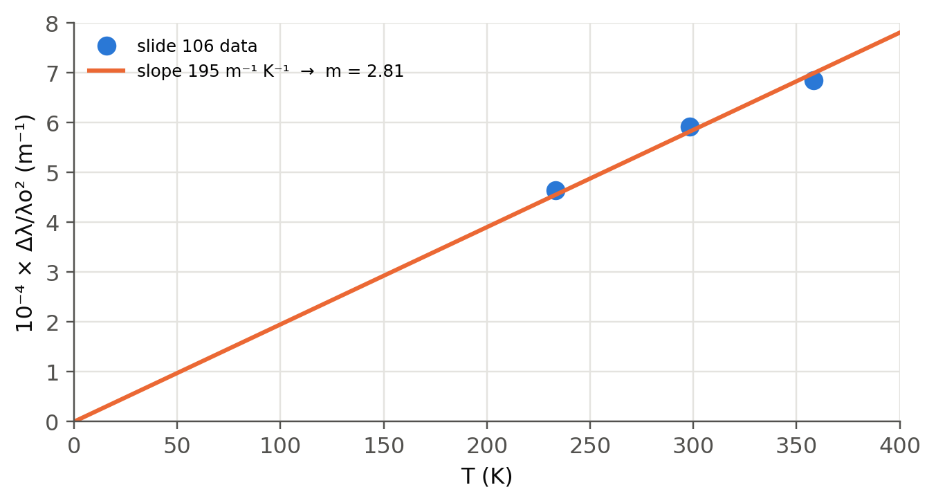
> **Slides 105–106.** An AlGaAs LED has $\lambda_o$ = 804, 822, 837 nm and $\Delta\lambda$ = 30, 40, 48 nm at −40, 25 and 85 °C.
> Plot $\Delta\lambda/\lambda_o^2$ against $T$ and find $m$ in $\Delta(h\nu)=mk_BT$.
> **Slides 107–108.** Shift of the peak of a GaAs LED cooled from 25 °C to −25 °C (Varshni: $E_{go}=1.519$ eV,
> $A=5.41\times10^{-4}$ eV/K, $B=204$ K).
```{python}
#| label: fig-m
#| fig-cap: "Slides 105–106: Δλ/λo² against T for the AlGaAs LED, with the best line forced through the origin. The slope gives m ≈ 2.8."
T = np.array([-40, 25, 85]) + 273.15
lam0 = np.array([804, 822, 837])*1e-9; dlam = np.array([30, 40, 48])*1e-9
y = dlam/lam0**2
slope = np.sum(y*T)/np.sum(T**2)                       # least squares through the origin
m = slope*sl.h*sl.c0/sl.kB
fig, ax = plt.subplots(figsize=(7, 3.4))
ax.plot(T, y*1e-4, "o", ms=8, label="slide 106 data")
Tl = np.linspace(0, 400, 10); ax.plot(Tl, slope*Tl*1e-4, label=f"slope {slope:.0f} m⁻¹ K⁻¹  →  m = {m:.2f}")
ax.set(xlabel="T (K)", ylabel="10⁻⁴ × Δλ/λo² (m⁻¹)", xlim=(0, 400), ylim=(0, 8)); ax.legend(fontsize=8); plt.show()
```
```{python}
#| label: tbl-spectrum-ex
#| tbl-cap: "Slides 103–108 recomputed with CODATA constants. The slide values are 107 nm, m = 2.81, 864.2 nm, 852.4 nm and 11.8 nm."
Eg298, Eg248 = sl.varshni(298, *sl.VARSHNI["GaAs"]), sl.varshni(248, *sl.VARSHNI["GaAs"])
l298 = sl.wavelength_from_eV(Eg298 + sl.kT(298)/2); l248 = sl.wavelength_from_eV(Eg248 + sl.kT(248)/2)
hc_slide = 3e8*6.626e-34/1.602e-19                     # constants used on slide 107
pd.DataFrame({"value": {
    "Δλ of a 1310 nm LED at 300 K, m = 3 (slide 104)": f"{sl.led_linewidth(1310e-9)*1e9:.1f} nm",
    "same with the ideal width m = 1.8": f"{sl.led_linewidth(1310e-9, m=1.8)*1e9:.1f} nm",
    "m from the AlGaAs data (slide 105)": f"{m:.2f}",
    "E_g(298 K) of GaAs": f"{Eg298:.4f} eV",
    "λo at 298 K, hc/(E_g + kT/2)": f"{l298*1e9:.1f} nm  (slide constants: {hc_slide/(Eg298 + sl.kT(298)/2)*1e9:.1f} nm)",
    "E_g(248 K)": f"{Eg248:.4f} eV",
    "λo at 248 K": f"{l248*1e9:.1f} nm  (slide constants: {hc_slide/(Eg248 + sl.kT(248)/2)*1e9:.1f} nm)",
    "shift for −50 K": f"{(l298 - l248)*1e9:.1f} nm = {(l298 - l248)*1e9/50:.2f} nm/K"}})
```
The 0.9 nm offset in the absolute wavelengths comes from the rounded constants on slide 107 ($c=3\times10^8$ m/s and
$h=6.626\times10^{-34}$ J s give $hc/e=1.2409$ eV µm instead of 1.2398). The shift of 0.24 nm/K is unaffected. Measuring this
shift is a practical way to monitor the **junction temperature** of a power LED.
## Temperature dependence (slides 101–102)
```{python}
#| label: fig-spectra-T
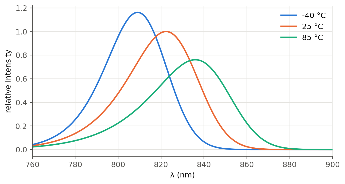
#| fig-cap: "Model spectra of an Al₀.₀₅Ga₀.₉₅As LED at −40, 25 and 85 °C (ideal shape, Varshni gap, 20 meV Gaussian broadening, intensity scaled by a typical −0.5 %/K efficiency drop), normalised to the 25 °C peak as in slide 101."
E = np.linspace(1.35, 1.75, 3000)
def spectrum(TC, sigma=0.020, off=0.059):           # off: Al-induced gap increase, puts the 25 °C peak at 822 nm
    T = TC + 273.15
    Eg = sl.varshni(T, *sl.VARSHNI["GaAs"]) + off
    S = sl.led_spectrum(E, Eg, T)
    g = np.exp(-((E - E.mean())**2)/(2*sigma**2)); S = np.convolve(S, g/g.sum(), mode="same")
    return S*(1 - 0.005*(TC - 25))
ref = spectrum(25).max()
fig, ax = plt.subplots(figsize=(7.5, 3.8))
rows = {}
for TC in (-40, 25, 85):
    S = spectrum(TC)/ref; lam = sl.wavelength_from_eV(E)*1e9
    ax.plot(lam, S, label=f"{TC} °C")
    half = lam[S >= S.max()/2]
    rows[f"{TC} °C"] = {"λo (nm)": round(lam[np.argmax(S)], 1), "Δλ FWHM (nm)": round(half.max() - half.min(), 1)}
ax.set(xlabel="λ (nm)", ylabel="relative intensity", xlim=(760, 900)); ax.legend(); plt.show()
pd.DataFrame(rows)
```
The model reproduces the trend of slide 101: about +0.25 nm/K in peak wavelength and a width that grows roughly as $T$ (the
measured 30–48 nm also include alloy broadening).
## Degenerately doped junctions (slide 109)
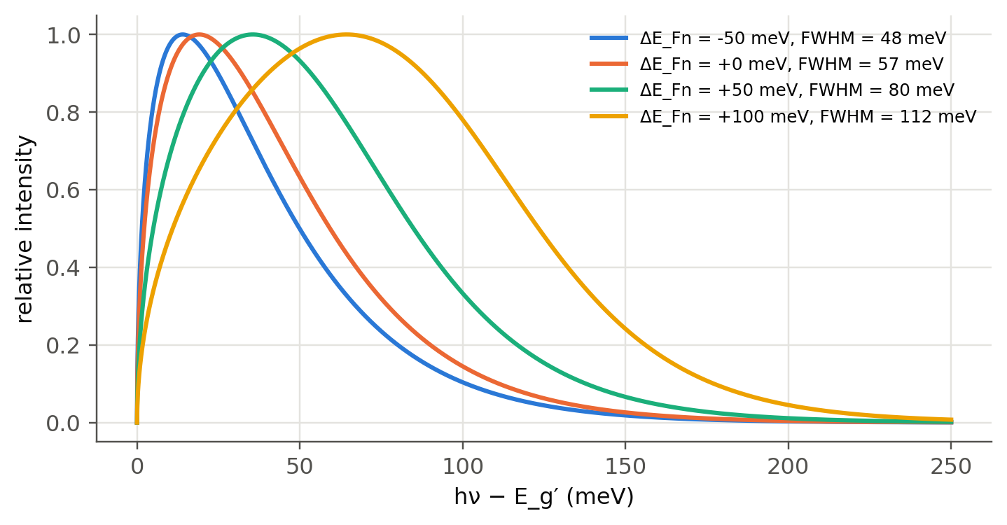
In a heavily doped n⁺ region $E_{Fn}$ lies inside the CB. All states up to $E_{Fn}$ can recombine, the spectrum widens to about
$\Delta E_{Fn}+1.5k_BT$, and the effective gap shrinks (band-gap narrowing):
```{python}
#| label: fig-degenerate
#| fig-cap: "Emission from a degenerately doped n⁺ region (holes non-degenerate): I(hν) ∝ (hν − E_g′)^{1/2} f_n(E). As E_Fn moves into the band (ΔE_Fn = E_Fn − E_c′), the spectrum becomes a flat-topped band of width ≈ ΔE_Fn + 1.5kT."
kT = sl.kT(300); x = np.linspace(0, 0.25, 3000)
fig, ax = plt.subplots(figsize=(7.5, 3.6))
for dEF in (-0.05, 0.0, 0.05, 0.10):
    I = np.sqrt(x)/(1 + np.exp((x - dEF)/kT))
    half = x[I >= I.max()/2]
    ax.plot(x*1e3, I/I.max(), label=f"ΔE_Fn = {dEF*1e3:+.0f} meV, FWHM = {(half.max() - half.min())*1e3:.0f} meV")
ax.set(xlabel="hν − E_g′ (meV)", ylabel="relative intensity"); ax.legend(fontsize=8); plt.show()
```
::: {.callout-tip collapse="true"}
## Going deeper
- **Van Roosbroeck–Shockley.** Derive the spontaneous emission spectrum from the absorption coefficient $\alpha(h\nu)$ and detailed
balance. With $\alpha\propto\sqrt{h\nu-E_g}$ you recover the shape used here, multiplied by $\nu^2$.
- **Coherence length.** Combine the LED linewidth with Chapter 1: $l_c=\lambda^2/\Delta\lambda$. Compute it for the 1310 nm LED and
explain why LEDs are used in OCT (superluminescent diodes) but not in long-haul links.
- **Chromatic dispersion.** A 1310 nm LED with $\Delta\lambda=107$ nm launched into a fiber with $D=2$ ps/(nm km) spreads by 0.2 ns/km.
Use the Chapter 2 link simulator to find the maximum bit rate.
- **Urbach tail.** Real absorption edges have an exponential tail $\exp[(h\nu-E_g)/E_U]$. Add it to the model and fit the measured
spectrum of a lab LED.
:::
::: {.callout-note collapse="true"}
## Complements
- Kasap, *Optoelectronics and Photonics*, sec. 3.11; Schubert, *Light-Emitting Diodes*, ch. 5 (spontaneous emission), ch. 6 (spectrum).
- Y. P. Varshni, "Temperature dependence of the energy gap in semiconductors", *Physica* 34, 149 (1967).
:::
## Try it yourself
1. What is the linewidth of a 460 nm InGaN LED at 300 K according to the $3k_BT$ rule? Compare with a typical datasheet (~20 nm).
2. Use the explorer to find the temperature rise that shifts a GaAs LED by 5 nm.
3. Redo the fit of slides 105–106 without forcing the line through the origin. What does the intercept mean physically?
4. Estimate the energy shift of the peak for a degenerate n⁺ region with $\Delta E_{Fn}=50$ meV.