# The pn junction at equilibrium {#sec-junction}
[](https://colab.research.google.com/github/{{< var github_user >}}/{{< var repo >}}/blob/main/{{< var subdir >}}/notebooks/junction.ipynb){.colab-link} Run this chapter's code in Google Colab (no installation).
```{python}
#| include: false
import numpy as np
import matplotlib.pyplot as plt
import pandas as pd
import scipy.sparse as sp
from scipy.sparse.linalg import spsolve
import semilib as sl
sl.use_style()
CM3 = sl.CM3
```
*Slides 40–47 (space charge layer, Poisson's equation, built-in field and voltage, depletion widths, law of the junction)
and 82–85 (band diagrams of the junction, built-in voltage from the band diagram).*
## Key relations
When p- and n-type regions touch, electrons and holes diffuse across the junction and recombine. They leave behind ionised
acceptors ($-eN_a$) on the p side and ionised donors ($+eN_d$) on the n side: the **space charge layer** (SCL) or depletion
region (slide 40). Its charge creates a field that stops further diffusion. Poisson's equation links charge, field and
potential (slide 41):
$$
\frac{d^2V}{dx^2}=-\frac{dE}{dx}=-\frac{\rho_\text{net}(x)}{\varepsilon},\qquad \varepsilon=\varepsilon_0\varepsilon_r .
$$
For an abrupt junction in the **depletion approximation** (slides 43–44):
$$
N_aW_p=N_dW_n,\qquad E_o=-\frac{eN_dW_n}{\varepsilon}=-\frac{eN_aW_p}{\varepsilon},\qquad V_o=-\tfrac12E_oW_o,
$$
$$
V_o=\frac{k_BT}{e}\ln\frac{N_aN_d}{n_i^2},\qquad W=\left[\frac{2\varepsilon(N_a+N_d)(V_o-V)}{eN_aN_d}\right]^{1/2}.
$$
$V$ is the applied voltage (positive for forward bias). In equilibrium the Fermi level is flat (slide 45) and the minority and
majority concentrations on the two sides obey the **law of the junction** (slides 46–47), Boltzmann statistics applied across
the barrier $eV_o$:
$$
\frac{p_{no}}{p_{po}}=\exp\!\left(-\frac{eV_o}{k_BT}\right),\qquad \frac{n_{po}}{n_{no}}=\exp\!\left(-\frac{eV_o}{k_BT}\right).
$$
## Junction explorer
```{ojs}
//| echo: false
matJ = ({
  Si:   {Eg: 1.11, ni: 1.0e10, er: 11.8},
  Ge:   {Eg: 0.66, ni: 2.3e13, er: 16.0},
  GaAs: {Eg: 1.42, ni: 2.1e6,  er: 13.0},
  InP:  {Eg: 1.35, ni: 3.0e7,  er: 12.6}
})
viewof jn = Inputs.form({
  mat: Inputs.select(Object.keys(matJ), {value: "Si", label: "material"}),
  lNa: Inputs.range([14, 19], {value: 17, step: 0.05, label: "log₁₀ N_a, p side (cm⁻³)"}),
  lNd: Inputs.range([14, 19], {value: 16, step: 0.05, label: "log₁₀ N_d, n side (cm⁻³)"}),
  V: Inputs.range([-10, 1.2], {value: 0, step: 0.01, label: "applied voltage V (V)"})
})
```
```{ojs}
//| echo: false
jnOut = {
  const m = matJ[jn.mat], q = 1.602176634e-19, eps = m.er*8.8541878e-12, kT = 0.025852;
  const Na = 10**jn.lNa*1e6, Nd = 10**jn.lNd*1e6, ni = m.ni*1e6;
  const Vo = kT*Math.log(Na*Nd/ni**2), V = Math.min(jn.V, Vo - 0.02);
  const W = Math.sqrt(2*eps*(Na + Nd)*(Vo - V)/(q*Na*Nd)), Wn = W*Na/(Na + Nd), Wp = W*Nd/(Na + Nd);
  const Eo = q*Nd*Wn/eps, L = 1.5*W, pts = [];
  // electron PE: E_c(x) = E_c(p side) − e V(x); the n side lies e(Vo − V) lower
  const EcP = m.Eg/2 + kT*Math.log(Na/ni);      // Ec − EF on the neutral p side (E_Fi taken at mid-gap)
  for (let i = 0; i <= 600; i++) {
    const x = -L + 2*L*i/600;
    let rho = 0, E = 0, phi = 0;
    if (x <= -Wp) { phi = 0; }
    else if (x < 0) { rho = -q*Na; E = -q*Na*(x + Wp)/eps; phi = q*Na*(x + Wp)**2/(2*eps); }
    else if (x < Wn) { rho = q*Nd; E = -q*Nd*(Wn - x)/eps; phi = (Vo - V) - q*Nd*(Wn - x)**2/(2*eps); }
    else { phi = Vo - V; }
    pts.push({x: x*1e6, rho: rho/1e6/q, E: E/1e5, Ec: EcP - phi, Ev: EcP - m.Eg - phi});
  }
  return {pts, Vo, V, W, Wn, Wp, Eo, Eg: m.Eg, clipped: jn.V > Vo - 0.02};
}
Plot.plot({
  width: Math.min(width, 1050), height: 190, marginLeft: 70, x: {label: null},
  y: {label: "ρ/e (cm⁻³)", grid: true, tickFormat: "~e"},
  marks: [Plot.areaY(jnOut.pts, {x: "x", y: "rho", fill: "#2a78d6", fillOpacity: 0.3}), Plot.line(jnOut.pts, {x: "x", y: "rho", stroke: "#2a78d6", strokeWidth: 2}), Plot.ruleY([0])]
})
```
```{ojs}
//| echo: false
Plot.plot({
  width: Math.min(width, 1050), height: 190, marginLeft: 70, x: {label: null},
  y: {label: "E (kV/cm)", grid: true},
  marks: [Plot.areaY(jnOut.pts, {x: "x", y: "E", fill: "#eb6834", fillOpacity: 0.3}), Plot.line(jnOut.pts, {x: "x", y: "E", stroke: "#eb6834", strokeWidth: 2}), Plot.ruleY([0])]
})
```
```{ojs}
//| echo: false
Plot.plot({
  width: Math.min(width, 1050), height: 260, marginLeft: 70, x: {label: "x (µm), metallurgical junction at 0, p side on the left"},
  y: {label: "electron energy (eV)", grid: true},
  marks: [
    Plot.line(jnOut.pts, {x: "x", y: "Ec", stroke: "#2a78d6", strokeWidth: 2}),
    Plot.line(jnOut.pts, {x: "x", y: "Ev", stroke: "#eb6834", strokeWidth: 2}),
    Plot.line([{x: jnOut.pts[0].x, y: 0}, {x: 0, y: 0}], {x: "x", y: "y", stroke: "#4a3aa7", strokeDasharray: "6,4", strokeWidth: 1.5}),
    Plot.line([{x: 0, y: jnOut.V}, {x: jnOut.pts[jnOut.pts.length - 1].x, y: jnOut.V}], {x: "x", y: "y", stroke: "#4a3aa7", strokeDasharray: "6,4", strokeWidth: 1.5}),
    Plot.text([{x: jnOut.pts[0].x, y: 0, t: "E_Fp"}, {x: jnOut.pts[jnOut.pts.length - 1].x, y: jnOut.V, t: "E_Fn"}], {x: "x", y: "y", text: "t", dy: -8, textAnchor: "middle", fill: "#4a3aa7"}),
    Plot.text([{x: jnOut.pts[0].x, y: jnOut.pts[0].Ec, t: "E_c"}, {x: jnOut.pts[0].x, y: jnOut.pts[0].Ev, t: "E_v"}], {x: "x", y: "y", text: "t", dy: -8, dx: 12, fill: "#0b0b0b"})
  ]
})
```
```{ojs}
//| echo: false
html`<div class="result-box">V<sub>o</sub> = <b>${jnOut.Vo.toFixed(3)} V</b> · W = <b>${(jnOut.W*1e6).toFixed(3)} µm</b>
(W<sub>p</sub> = ${(jnOut.Wp*1e6).toFixed(3)} µm, W<sub>n</sub> = ${(jnOut.Wn*1e6).toFixed(3)} µm) ·
peak field |E<sub>o</sub>| = <b>${(jnOut.Eo/1e5).toFixed(1)} kV/cm</b> · barrier e(V<sub>o</sub> − V) = ${(jnOut.Vo - jnOut.V).toFixed(3)} eV
${jnOut.clipped ? html`<br><b>V ≥ V<sub>o</sub>: the depletion approximation no longer applies; V clipped to V<sub>o</sub> − 0.02 V.</b>` : ""}</div>`
```
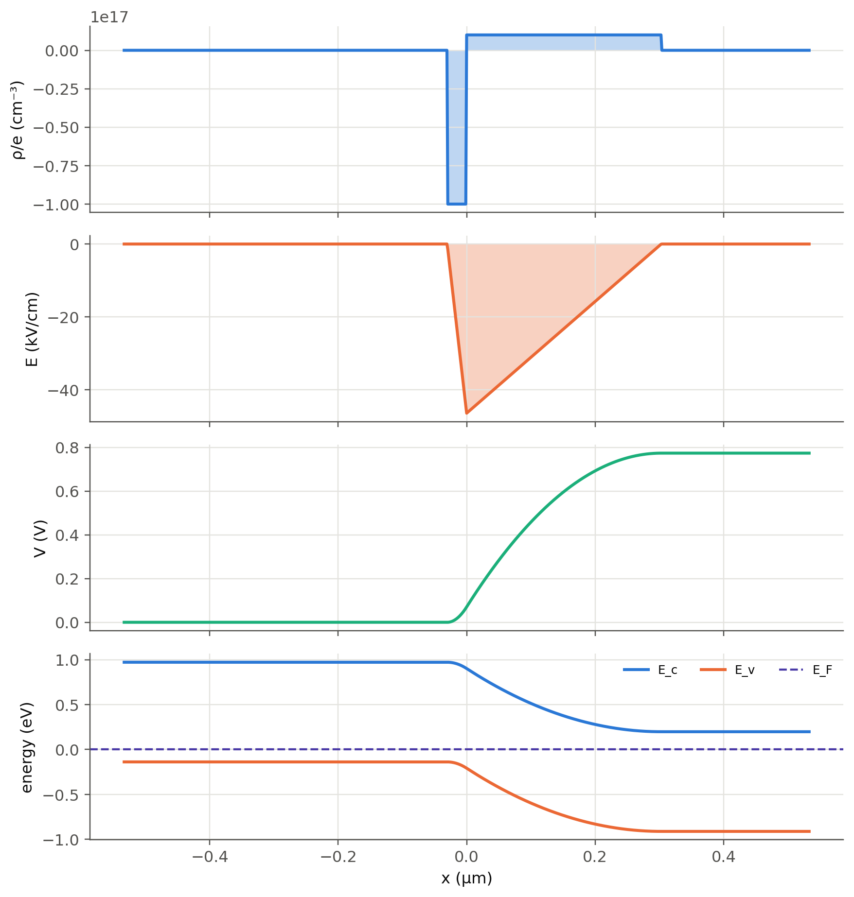
In the band diagram the energy axis is electron energy, referenced to the p-side Fermi level. Forward bias ($V>0$) raises the
n-side Fermi level by $eV$ and lowers the barrier. Reverse bias does the opposite and widens the SCL. The depletion region
extends mostly into the **lightly doped side**: try $N_a=10^{19}$, $N_d=10^{15}$ cm⁻³ (a p⁺n junction).
## Worked numbers, recomputed
```{python}
#| label: tbl-junction
#| tbl-cap: "Built-in voltage, depletion widths and peak field for three abrupt junctions at 300 K. The GaAs row is the device of slides 75–79 (V_o = 1.27 V and W = 0.116 µm at 0.8 V forward bias on the slides)."
cases = {"GaAs, Na = Nd = 1e17, V = 0 (slide 78)": ("GaAs", 1e17, 1e17, 0.0),
         "GaAs, Na = Nd = 1e17, V = 0.80 V (slide 79)": ("GaAs", 1e17, 1e17, 0.80),
         "Si p⁺n, Na = 1e18, Nd = 1e16, V = 0": ("Si", 1e18, 1e16, 0.0),
         "Si p⁺n, same, V = −10 V": ("Si", 1e18, 1e16, -10.0),
         "Ge, Na = 1e17, Nd = 1e16, V = 0": ("Ge", 1e17, 1e16, 0.0)}
rows = {}
for k, (m, Na, Nd, V) in cases.items():
    p = sl.MATERIALS[m]
    Vo = sl.built_in_voltage(Na*CM3, Nd*CM3, p["ni"])
    d = sl.depletion(Na*CM3, Nd*CM3, p["eps_r"], Vo, V)
    rows[k] = {"V_o (V)": round(Vo, 3), "W (µm)": round(d["W"]*1e6, 4), "W_p (µm)": round(d["Wp"]*1e6, 4),
               "W_n (µm)": round(d["Wn"]*1e6, 4), "|E_o| (kV/cm)": round(d["Eo"]/1e5, 1)}
pd.DataFrame(rows).T
```
## Charge, field, potential and bands {#sec-junction-profile}
```{python}
#| label: fig-junction-profile
#| fig-cap: "Si junction with N_a = 10¹⁷ and N_d = 10¹⁶ cm⁻³ at equilibrium (slides 40 and 42): net space charge, field (triangular), electrostatic potential (two parabolas) and the resulting band diagram, where E_c(x) = E_c(p) − eV(x). The field peaks at the metallurgical junction."
Na, Nd = 1e17*CM3, 1e16*CM3
ni = sl.MATERIALS["Si"]["ni"]
Vo = sl.built_in_voltage(Na, Nd, ni)
x, rho, E, V = sl.junction_profile(Na, Nd, 11.8, Vo)
kT = sl.kT(); Eg = 1.11
EcP = Eg/2 + kT*np.log(Na/ni)                     # Ec − EF on the neutral p side (E_Fi at mid-gap)
fig, ax = plt.subplots(4, 1, figsize=(8, 8.5), sharex=True)
ax[0].fill_between(x*1e6, rho/sl.qe/CM3, alpha=0.3, lw=0); ax[0].plot(x*1e6, rho/sl.qe/CM3); ax[0].set_ylabel("ρ/e (cm⁻³)")
ax[1].fill_between(x*1e6, E/1e5, alpha=0.3, lw=0, color=sl.PALETTE[1]); ax[1].plot(x*1e6, E/1e5, color=sl.PALETTE[1]); ax[1].set_ylabel("E (kV/cm)")
ax[2].plot(x*1e6, V, color=sl.PALETTE[2]); ax[2].set_ylabel("V (V)")
ax[3].plot(x*1e6, EcP - V, label="E_c"); ax[3].plot(x*1e6, EcP - Eg - V, label="E_v", color=sl.PALETTE[1])
ax[3].axhline(0, color=sl.PALETTE[6], ls="--", lw=1.4, label="E_F"); ax[3].set(ylabel="energy (eV)", xlabel="x (µm)")
ax[3].legend(fontsize=8, ncol=3, loc="upper right")
plt.tight_layout(); plt.show()
```
## Beyond the depletion approximation: solving Poisson exactly {#sec-poisson}
The depletion approximation assumes a sharp edge between "fully depleted" and "neutral". In reality the mobile carriers follow
Boltzmann statistics in the local potential, $n=n_ie^{\psi/V_T}$, $p=n_ie^{-\psi/V_T}$, and Poisson's equation becomes nonlinear:
$$
\frac{d^2\psi}{dx^2}=-\frac{e}{\varepsilon}\left[n_ie^{-\psi/V_T}-n_ie^{\psi/V_T}+N_d(x)-N_a(x)\right].
$$
A few Newton iterations on a finite-difference grid solve it (this is the core of every device simulator):
```{python}
#| label: fig-poisson
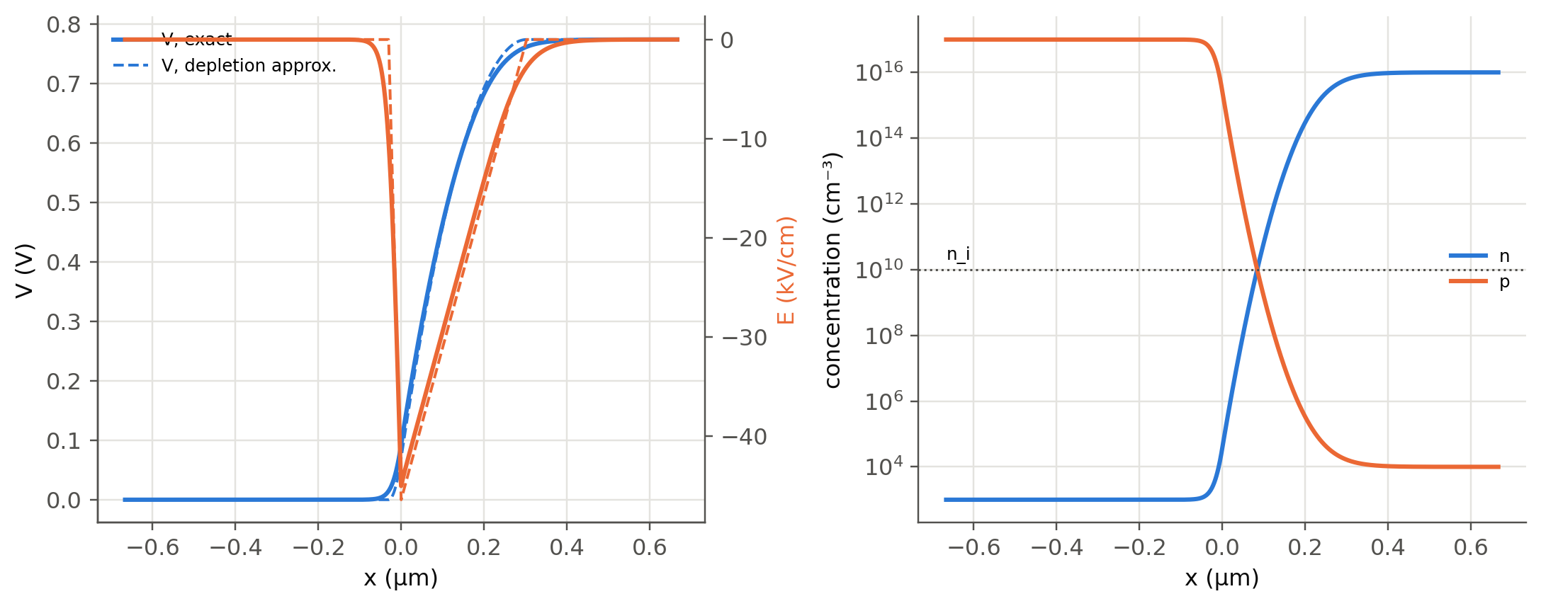
#| fig-cap: "Exact (Poisson–Boltzmann, solid) versus depletion-approximation (dashed) solution for the same Si junction. Left: potential and field agree except for soft edges a few Debye lengths wide. Right: carrier concentrations on a log scale (slide 40c): the majority carriers drop smoothly across the SCL and n·p = n_i² everywhere at equilibrium."
def poisson_pn(Na, Nd, eps_r, ni, T=300.0, L=None, N=2001, tol=1e-10):
    Vt, eps = sl.kT(T), eps_r*sl.eps0
    Vo = sl.built_in_voltage(Na, Nd, ni, T)
    L = L or 2*sl.depletion(Na, Nd, eps_r, Vo)["W"]
    x = np.linspace(-L, L, N); dx = x[1] - x[0]
    Nnet = np.where(x < 0, -Na, Nd)
    u = np.where(x < 0, -np.log(Na/ni), np.log(Nd/ni))          # ψ/Vt, start from neutral values
    c = sl.qe*ni/(eps*Vt)*dx**2
    for _ in range(200):
        lap = np.zeros(N); lap[1:-1] = u[2:] - 2*u[1:-1] + u[:-2]
        R = lap + c*(np.exp(-u) - np.exp(u) + Nnet/ni); R[0] = R[-1] = 0
        main = -2 - c*(np.exp(-u) + np.exp(u)); main[0] = main[-1] = 1
        J = sp.diags([np.r_[np.ones(N-2), 0], main, np.r_[0, np.ones(N-2)]], [-1, 0, 1], format="csc")
        du = spsolve(J, -R); du = np.clip(du, -1, 1)              # damped Newton step
        u += du
        if np.max(abs(du)) < tol: break
    psi = u*Vt
    return x, psi - psi[0], -np.gradient(psi, x), ni*np.exp(u), ni*np.exp(-u)

xs, Vex, Eex, n, p = poisson_pn(Na, Nd, 11.8, ni)
xd, _, Ed, Vd = sl.junction_profile(Na, Nd, 11.8, Vo, npts=2001, span=2)
fig, ax = plt.subplots(1, 2, figsize=(10, 4))
ax[0].plot(xs*1e6, Vex, label="V, exact"); ax[0].plot(xd*1e6, Vd, "--", color=sl.PALETTE[0], lw=1.3, label="V, depletion approx.")
a2 = ax[0].twinx(); a2.plot(xs*1e6, Eex/1e5, color=sl.PALETTE[1]); a2.plot(xd*1e6, Ed/1e5, "--", color=sl.PALETTE[1], lw=1.3)
a2.set_ylabel("E (kV/cm)", color=sl.PALETTE[1]); a2.spines["right"].set_visible(True); a2.grid(False)
ax[0].set(xlabel="x (µm)", ylabel="V (V)"); ax[0].legend(fontsize=8, loc="upper left")
ax[1].semilogy(xs*1e6, n/CM3, label="n"); ax[1].semilogy(xs*1e6, p/CM3, label="p")
ax[1].axhline(ni/CM3, color=sl.INK2, ls=":", lw=1); ax[1].text(xs[0]*1e6, ni/CM3*2, "n_i", fontsize=8)
ax[1].set(xlabel="x (µm)", ylabel="concentration (cm⁻³)"); ax[1].legend(fontsize=8)
plt.tight_layout(); plt.show()
LD = np.sqrt(11.8*sl.eps0*sl.kT()/(sl.qe*Nd))
print(f"V_o: exact {Vex[-1]:.4f} V, formula {Vo:.4f} V;  Debye length on the n side L_D = {LD*1e9:.0f} nm")
print(f"law of the junction: p_n0/p_p0 = {p[-1]/p[0]:.3e},  exp(−eVo/kT) = {np.exp(-Vo/sl.kT()):.3e}")
```
The potential step of the exact solution equals $V_o$ to four digits, and the ratio of hole concentrations on the two sides
reproduces the law of the junction: slides 44 and 46 describe the same physics. The depletion edges are smeared over a few
**Debye lengths** $L_D=\sqrt{\varepsilon k_BT/e^2N}$.
## Built-in voltage from the band diagram (slides 82–83)
Before contact the two Fermi levels differ; after contact they align and the bands bend by exactly that difference:
$eV_o=E_{Fn}-E_{Fp}=\Phi_p-\Phi_n$. With the electron affinity $\chi$ of Table 3.1 the work functions follow from the position
of $E_F$ in each region:
```{python}
#| label: tbl-workfunction
#| tbl-cap: "Si, Na = 10¹⁷ and Nd = 10¹⁶ cm⁻³: work functions Φ = χ + (E_c − E_F) of the separated regions (slide 24) and the built-in voltage from their difference (slide 83)."
p = sl.MATERIALS["Si"]
EcEFn = -sl.kT()*np.log(Nd/p["Nc"])                  # (3.9.1)
EcEFp = -sl.kT()*np.log(p["ni"]**2/(Na*p["Nc"]))     # (3.9.2)
pd.DataFrame({"n side": {"E_c − E_F (eV)": EcEFn, "Φ = χ + E_c − E_F (eV)": p["chi"] + EcEFn},
              "p side": {"E_c − E_F (eV)": EcEFp, "Φ = χ + E_c − E_F (eV)": p["chi"] + EcEFp},
              "eV_o = Φ_p − Φ_n": {"E_c − E_F (eV)": np.nan, "Φ = χ + E_c − E_F (eV)": EcEFp - EcEFn}}).T.round(3)
```
::: {.callout-tip collapse="true"}
## Going deeper
- **Linearly graded junction.** Implanted and diffused junctions are graded, $N_d-N_a=ax$. Show that $W\propto(V_o-V)^{1/3}$ and
check it with `poisson_pn` by changing `Nnet`.
- **Breakdown.** The peak field limits the reverse voltage. Si breaks down by avalanche near 3–5×10⁵ V/cm. Use the explorer
to estimate the breakdown voltage of a p⁺n junction with $N_d=10^{15}$ and $10^{17}$ cm⁻³. Which one would you choose for an
avalanche photodiode (Ch. 5)?
- **pin structure.** Insert an intrinsic layer of width $d$ between p and n. The field becomes nearly uniform. Modify
`poisson_pn` and compare with the p–n case. This is the photodiode geometry of Chapter 5.
- **Under bias.** Extend the Newton solver with two quasi-Fermi levels and the drift–diffusion equations (Scharfetter–Gummel):
a 1D device simulator in 100 lines. Packages such as `solcore` and `devsim` do this.
:::
::: {.callout-note collapse="true"}
## Complements
- Kasap, *Optoelectronics and Photonics*, sec. 3.3; Sze & Ng, ch. 2 (pn junctions).
- S. Selberherr, *Analysis and Simulation of Semiconductor Devices* (Springer, 1984): numerical methods behind device simulators.
- DEVSIM: open-source TCAD in Python, <https://devsim.org>.
:::
## Try it yourself
1. A Si p⁺n junction has $N_d=10^{15}$ cm⁻³. Find the reverse voltage at which $W$ reaches 10 µm (useful for a photodiode).
2. Why does the depletion layer of a p⁺n junction lie almost entirely on the n side? Show that $W_n/W\to1$ when $N_a\gg N_d$.
3. Compute $V_o$ for GaAs and Ge junctions with the same doping. Why does it scale roughly with $E_g$?
4. In `poisson_pn`, double the temperature to 600 K. What happens to $V_o$ and to the Debye tails?