# Quantum wells {#sec-qw}
[](https://colab.research.google.com/github/{{< var github_user >}}/{{< var repo >}}/blob/main/{{< var subdir >}}/notebooks/quantum-wells.ipynb){.colab-link} Run this chapter's code in Google Colab (no installation).
```{python}
#| include: false
import numpy as np
import matplotlib.pyplot as plt
import pandas as pd
import semilib as sl
sl.use_style()
```
*Slides 110–113: single quantum well, quantised levels, two-dimensional density of states, worked example on the levels of a
GaAs/AlGaAs well, multiple quantum wells.*
## Key relations
A layer of a narrow-gap semiconductor thinner than about 20 nm, sandwiched between wide-gap barriers, confines electrons along
$x$ (slide 110). The motion along $x$ is quantised, while the motion in the plane ($y$, $z$) stays free (slide 111):
$$
E_n=E_c+\frac{h^2n^2}{8m_e^*d^2}+\frac{\hbar^2k_y^2}{2m_e^*}+\frac{\hbar^2k_z^2}{2m_e^*},\qquad n=1,2,3,\dots
$$
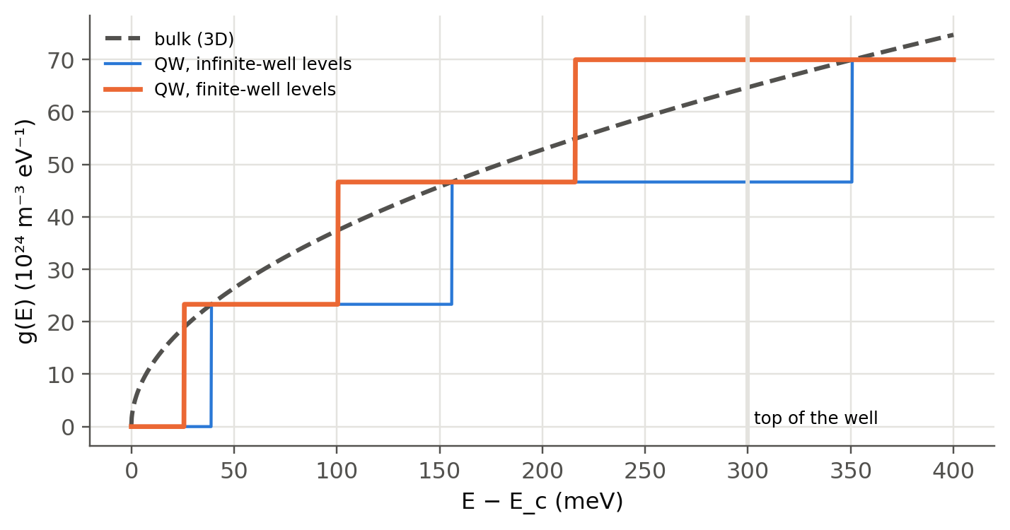
The first term is the infinite-well result. Each level $E_n$ starts a **sub-band** whose density of states per unit area is
constant, $g_{2D}=m^*/\pi\hbar^2$. The total DOS is a **staircase** that touches the bulk $\sqrt E$ curve at each step (slide
110c). Carriers collect at the bottom of the lowest sub-band, so the emission is narrower and occurs at
$$
h\nu=E_{g1}+E_1+E_1'
$$
(electron plus hole confinement energies). The well width becomes a design parameter for the wavelength.
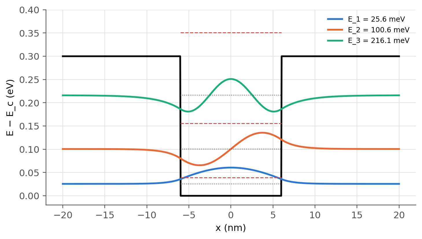
For a well of finite depth $\Delta E_c$ the wavefunction leaks into the barriers and the levels are lower. They follow from matching
$\psi$ and $\psi'/m^*$ at the interfaces:
$$
\text{even: }\ \frac{k}{m_w}\tan\frac{kd}{2}=\frac{\kappa}{m_b},\qquad
\text{odd: }\ -\frac{k}{m_w}\cot\frac{kd}{2}=\frac{\kappa}{m_b},\qquad
k=\frac{\sqrt{2m_wE}}{\hbar},\ \ \kappa=\frac{\sqrt{2m_b(\Delta E_c-E)}}{\hbar}.
$$
## Finite-well solver
```{ojs}
//| echo: false
viewof qw = Inputs.form({
  d: Inputs.range([1, 30], {value: 12, step: 0.5, label: "well width d (nm)"}),
  V0: Inputs.range([0.02, 0.6], {value: 0.30, step: 0.01, label: "barrier height ΔE_c (eV)"}),
  mw: Inputs.range([0.02, 0.5], {value: 0.067, step: 0.001, label: "well effective mass m_w*/m_e"}),
  mb: Inputs.range([0.02, 0.5], {value: 0.067, step: 0.001, label: "barrier effective mass m_b*/m_e"})
})
```
```{ojs}
//| echo: false
qwOut = {
  const hbar = 1.054571817e-34, me = 9.1093837e-31, q = 1.602176634e-19, d = qw.d*1e-9, V0 = qw.V0;
  const k = E => Math.sqrt(2*qw.mw*me*E*q)/hbar, K = E => Math.sqrt(2*qw.mb*me*(V0 - E)*q)/hbar;
  const even = E => (k(E)/qw.mw)*Math.sin(k(E)*d/2) - (K(E)/qw.mb)*Math.cos(k(E)*d/2);
  const odd = E => (k(E)/qw.mw)*Math.cos(k(E)*d/2) + (K(E)/qw.mb)*Math.sin(k(E)*d/2);
  const levels = [];
  for (const [f, par] of [[even, 0], [odd, 1]]) {
    const N = 4000; let Ep = V0*1e-6, fp = f(Ep);
    for (let i = 1; i <= N; i++) {
      const E = V0*(1e-6 + (1 - 2e-6)*i/N), fe = f(E);
      if (fp*fe < 0) { let a = Ep, b = E; for (let j = 0; j < 60; j++) { const c = (a + b)/2; if (f(a)*f(c) <= 0) b = c; else a = c; } levels.push({E: (a + b)/2, par}); }
      Ep = E; fp = fe;
    }
  }
  levels.sort((a, b) => a.E - b.E);
  const inf = [1, 2, 3, 4].map(n => (6.62607015e-34*n)**2/(8*qw.mw*me*d*d)/q);
  const L = 1.5*qw.d, pot = [{x: -L, V: V0}, {x: -qw.d/2, V: V0}, {x: -qw.d/2, V: 0}, {x: qw.d/2, V: 0}, {x: qw.d/2, V: V0}, {x: L, V: V0}];
  const amp = 0.35*V0/Math.max(1, levels.length);
  const wf = levels.flatMap((lv, n) => {
    const kk = k(lv.E)*1e-9, KK = K(lv.E)*1e-9, out = [];
    for (let i = 0; i <= 400; i++) { const x = -L + 2*L*i/400; let psi;
      if (Math.abs(x) <= qw.d/2) psi = lv.par === 0 ? Math.cos(kk*x) : Math.sin(kk*x);
      else { const edge = lv.par === 0 ? Math.cos(kk*qw.d/2) : Math.sin(kk*qw.d/2); psi = Math.sign(x)**lv.par*edge*Math.exp(-KK*(Math.abs(x) - qw.d/2)); }
      out.push({x, y: lv.E + amp*psi, n: `n = ${n + 1}`}); }
    return out; });
  const leak = levels.map(lv => { const kk = k(lv.E)*1e-9, KK = K(lv.E)*1e-9;
    let inside = 0, outside = 0; for (let i = 0; i <= 2000; i++) { const x = -3*L + 6*L*i/2000; let psi;
      if (Math.abs(x) <= qw.d/2) { psi = lv.par === 0 ? Math.cos(kk*x) : Math.sin(kk*x); inside += psi*psi; }
      else { const edge = lv.par === 0 ? Math.cos(kk*qw.d/2) : Math.sin(kk*qw.d/2); psi = edge*Math.exp(-KK*(Math.abs(x) - qw.d/2)); outside += psi*psi; } }
    return outside/(inside + outside); });
  return {levels, inf, pot, wf, L, leak};
}
Plot.plot({
  width: Math.min(width, 1050), height: 360, x: {label: "x (nm)", domain: [-qwOut.L, qwOut.L]},
  y: {label: "electron energy above E_c of the well (eV)", grid: true, domain: [-0.02, qw.V0*1.25]},
  color: {legend: true, range: ["#2a78d6", "#eb6834", "#1baf7a", "#eda100", "#e87ba4", "#008300", "#4a3aa7", "#e34948"]},
  marks: [
    Plot.line(qwOut.pot, {x: "x", y: "V", stroke: "#0b0b0b", strokeWidth: 2}),
    Plot.ruleY(qwOut.levels.map(l => l.E), {stroke: "#52514e", strokeDasharray: "2,3", x1: -qw.d/2, x2: qw.d/2}),
    Plot.ruleY(qwOut.inf.filter(e => e < qw.V0*1.25), {stroke: "#e34948", strokeWidth: 1, strokeDasharray: "6,3", x1: -qw.d/2, x2: qw.d/2}),
    Plot.line(qwOut.wf, {x: "x", y: "y", stroke: "n", strokeWidth: 2})
  ]
})
```
```{ojs}
//| echo: false
html`<div class="result-box">${qwOut.levels.length} bound level${qwOut.levels.length === 1 ? "" : "s"}:
${qwOut.levels.map((l, i) => `E<sub>${i+1}</sub> = <b>${(1000*l.E).toFixed(1)} meV</b> (${(100*qwOut.leak[i]).toFixed(0)} % in the barriers)`).join(" · ")}<br>
infinite well (red dashed): ${qwOut.inf.map((e, i) => `${(1000*e).toFixed(0)}`).join(", ")} meV</div>`
```
A finite well always has at least one bound state, however thin. Make the well narrow (2–3 nm): $E_1$ approaches the top, most of
the wavefunction sits in the barriers, and the infinite-well formula becomes useless.
## Worked example (slide 112), recomputed
> GaAs well between Al₀.₄Ga₀.₆As barriers, $\Delta E_c=0.30$ eV, $m_e^*=0.067m_e$, $d=12$ nm. Find $E_1$, $E_2$ for an infinite
> well and compare with the finite-well values 0.022, 0.088 and 0.186 eV quoted on the slide.
```{python}
#| label: tbl-qw
#| tbl-cap: "Electron levels (eV above E_c) of a 12 nm GaAs well with ΔE_c = 0.30 eV."
d, V0 = 12e-9, 0.30
pd.DataFrame({
    "infinite well (slide: 0.039, 0.156, 0.351)": sl.qw_infinite([1, 2, 3], d, 0.067),
    "finite well, m* = 0.067 everywhere": sl.qw_finite(d, V0, 0.067)[:3],
    "finite well, barrier mass 0.0919 (Al₀.₄Ga₀.₆As)": sl.qw_finite(d, V0, 0.067, 0.0919)[:3],
    "finite well, m* = 0.080 everywhere": sl.qw_finite(d, V0, 0.080)[:3],
    "slide (finite)": [0.022, 0.088, 0.186]}, index=["n = 1", "n = 2", "n = 3"]).round(4)
```
The infinite-well numbers match the slide. The finite-well values quoted on the slide are about 15 % lower than a direct solution
with $m^*=0.067m_e$, even with the heavier barrier mass of Al₀.₄Ga₀.₆As. They correspond to an effective mass close to $0.08m_e$
(non-parabolicity raises the mass of confined electrons, which may be the origin). The ratio infinite/finite is 1.5 for the
textbook parameters instead of the quoted 1.8. Either way the conclusion holds: the third level is bound in the real well but
above the barrier in the infinite model.
```{python}
#| label: fig-qw-wf
#| fig-cap: "The 12 nm GaAs/Al₀.₄Ga₀.₆As well: potential, finite-well levels and envelope wavefunctions (drawn at their energies). Red dashed: infinite-well levels."
x = np.linspace(-20e-9, 20e-9, 800)
lev = sl.qw_finite(d, V0, 0.067)
fig, ax = plt.subplots(figsize=(7.5, 4))
ax.plot(x*1e9, np.where(abs(x) <= d/2, 0, V0), color=sl.INK, lw=2)
for n, E in enumerate(lev):
    psi = sl.qw_wavefunction(x, E, d, V0, 0.067, parity=n % 2)
    ax.plot(x*1e9, E + 0.035*psi, label=f"E_{n+1} = {E*1e3:.1f} meV")
    ax.hlines(E, -d/2*1e9, d/2*1e9, color=sl.INK2, lw=0.8, ls=":")
for E in sl.qw_infinite([1, 2, 3], d, 0.067):
    ax.hlines(E, -d/2*1e9, d/2*1e9, color=sl.PALETTE[7], lw=1, ls="--")
ax.set(xlabel="x (nm)", ylabel="E − E_c (eV)", ylim=(-0.02, 0.4)); ax.legend(fontsize=8, loc="upper right"); plt.show()
```
## Tuning the wavelength with the well width
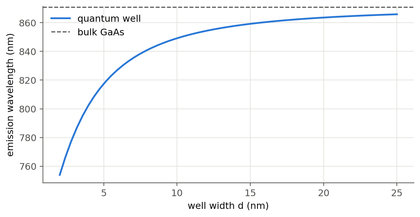
The emitted photon energy is $E_{g1}+E_1+E_1'$. For GaAs/Al₀.₃Ga₀.₇As ($\Delta E_g=0.374$ eV, split 67:33 between CB and VB,
heavy-hole mass $0.5m_e$):
```{python}
#| label: fig-qw-lambda
#| fig-cap: "Ground-state transition of a GaAs/Al₀.₃Ga₀.₇As quantum well (finite-well electron and heavy-hole levels, 300 K) versus well width. Thin wells push the emission from 870 nm toward 780 nm, the wavelength of CD lasers."
dEg = 1.247*0.3; dEc, dEv = 0.67*dEg, 0.33*dEg
widths = np.linspace(2e-9, 25e-9, 60)
E1 = np.array([sl.qw_finite(w, dEc, 0.067, 0.067 + 0.083*0.3)[0] for w in widths])
H1 = np.array([sl.qw_finite(w, dEv, 0.50, 0.50 + 0.14*0.3)[0] for w in widths])
Eph = 1.424 + E1 + H1
fig, ax = plt.subplots(figsize=(7.5, 3.6))
ax.plot(widths*1e9, sl.wavelength_from_eV(Eph)*1e9, label="quantum well")
ax.axhline(sl.wavelength_from_eV(1.424)*1e9, color=sl.INK2, ls="--", lw=1.2, label="bulk GaAs")
ax.set(xlabel="well width d (nm)", ylabel="emission wavelength (nm)"); ax.legend(); plt.show()
```
## The two-dimensional density of states (slide 110c)
```{python}
#| label: fig-dos2d
#| fig-cap: "Density of states per unit volume of a 12 nm GaAs well (staircase, each step m*/(πħ²d) at a finite-well level) compared with bulk GaAs. Each step lies on the bulk √E curve when the infinite-well levels are used; the finite well steps slightly earlier."
E = np.linspace(0, 0.4, 2000)
bulk = sl.dos_3d(E, 0.067)
step = 0.067*sl.me/(np.pi*sl.hbar**2*d)*sl.qe        # m^-3 eV^-1 per sub-band
stair_fin = step*np.sum([E >= e for e in sl.qw_finite(d, V0, 0.067)], axis=0)
stair_inf = step*np.sum([E >= e for e in sl.qw_infinite(np.arange(1, 6), d, 0.067)], axis=0)
fig, ax = plt.subplots(figsize=(7.5, 3.6))
ax.plot(E*1e3, bulk/1e24, label="bulk (3D)", color=sl.INK2, ls="--")
ax.plot(E*1e3, stair_inf/1e24, label="QW, infinite-well levels", lw=1.4)
ax.plot(E*1e3, stair_fin/1e24, label="QW, finite-well levels", lw=2.2)
ax.axvline(V0*1e3, color=sl.GRID, lw=2); ax.text(V0*1e3 + 3, 0.5, "top of the well", fontsize=8)
ax.set(xlabel="E − E_c (meV)", ylabel="g(E) (10²⁴ m⁻³ eV⁻¹)"); ax.legend(fontsize=8); plt.show()
```
The step-like DOS puts a finite number of states right at the band edge instead of zero. Carriers pile up at $E_1$, the
spectrum narrows, and less carrier density is needed to reach a given emission rate (or optical gain in lasers, Ch. 4).
## Single versus multiple quantum wells (slide 113)
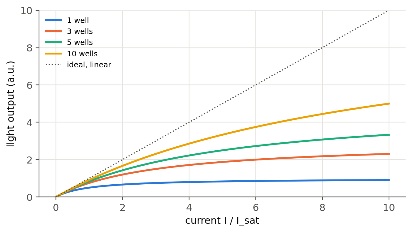
One thin well holds a limited number of carriers. At high current it saturates, carriers overflow into the barriers and the light
output becomes sublinear. Spreading the current over $N$ wells delays saturation. A minimal model gives each well a light output
$P_w=I_w/(1+I_w/I_\text{sat})$:
```{python}
#| label: fig-mqw
#| fig-cap: "Light output versus current for a single QW and for MQWs (model: each well saturates as I_w/(1 + I_w/I_sat), current shared equally). This reproduces the trend sketched on slide 113."
I = np.linspace(0, 10, 300)                          # in units of the saturation current of one well
fig, ax = plt.subplots(figsize=(7, 3.6))
for N in (1, 3, 5, 10):
    ax.plot(I, N*(I/N)/(1 + I/N), label=f"{N} well{'s' if N > 1 else ''}")
ax.plot(I, I, ":", color=sl.INK2, lw=1.2, label="ideal, linear")
ax.set(xlabel="current I / I_sat", ylabel="light output (a.u.)", ylim=(0, 10)); ax.legend(fontsize=8); plt.show()
```
In real InGaN MQWs the holes are heavy and travel poorly, so most of the light comes from the well nearest the p side. The extra
wells help less than this model suggests. This is one of the active research topics around "efficiency droop".
::: {.callout-tip collapse="true"}
## Going deeper
- **Shooting or matrix method.** Solve the Schrödinger equation on a grid (finite differences, `scipy.linalg.eigh_tridiagonal`)
for an arbitrary potential: a graded well, two coupled wells (splitting into bonding/antibonding states), or a superlattice
(minibands, compare with the Kronig–Penney model of @sec-kp).
- **Quantum-confined Stark effect.** Add a field $F$ to the potential, $V(x)-eFx$, and compute the red shift of $E_1$. This is the
principle of electro-absorption modulators (Ch. 6) and the origin of the wavelength shift in polar InGaN wells.
- **Excitons.** In a QW the electron–hole binding energy rises from 4 meV (bulk GaAs) to about 10 meV, which makes
room-temperature excitons visible in absorption. Estimate it with a 2D hydrogen model.
- **Quantum dots and wires.** Confine in two or three directions: the DOS becomes $1/\sqrt E$ peaks or delta functions. Plot all four
DOS types side by side.
:::
::: {.callout-note collapse="true"}
## Complements
- Kasap, *Optoelectronics and Photonics*, sec. 3.12; Schubert, *Light-Emitting Diodes*, ch. 7 and 12.
- P. Harrison and A. Valavanis, *Quantum Wells, Wires and Dots*, 4th ed. (Wiley, 2016): numerical methods with code.
- `nextnano` and the open-source Schrödinger–Poisson solver `aestimo` (Python) for real heterostructures.
:::
## Try it yourself
1. With the solver, find the width at which a GaAs well with $\Delta E_c=0.3$ eV acquires a third bound level.
2. Compute $E_1$ for an In₀.₂Ga₀.₈N well of 3 nm ($m^*=0.2$, $\Delta E_c\approx0.25$ eV). How much does confinement shift the emission?
3. Show that the number of bound states of a finite well is $\lceil (d/\pi\hbar)\sqrt{2m^*\Delta E_c}\,\rceil$ (equal masses).
4. Why must the barrier height exceed a few $k_BT$ for a QW LED to work at room temperature?