# Doping, Fermi level and conductivity {#sec-doping}
[](https://colab.research.google.com/github/{{< var github_user >}}/{{< var repo >}}/blob/main/{{< var subdir >}}/notebooks/doping.ipynb){.colab-link} Run this chapter's code in Google Colab (no installation).
```{python}
#| include: false
import numpy as np
import matplotlib.pyplot as plt
import pandas as pd
from scipy.optimize import brentq
import semilib as sl
sl.use_style()
CM3, CM2 = sl.CM3, sl.CM2
Si = sl.MATERIALS["Si"]
```
*Slides 18–32: drift mobility and conductivity, n- and p-type doping, band diagrams, compensation, degenerate
semiconductors, worked examples, bands in an applied field.*
## Key relations
A group-V atom (As, P) in Si gives a **donor** level a few tens of meV below $E_c$; at room temperature it is ionised and
$n\approx N_d$. A group-III atom (B) gives an **acceptor** just above $E_v$ and $p\approx N_a$ (slides 19–23). The minority
concentration follows from the mass action law. With both dopants present (**compensation**, slides 26–27):
$$
N_d>N_a:\ \ n=N_d-N_a,\ \ p=\frac{n_i^2}{N_d-N_a};\qquad N_a>N_d:\ \ p=N_a-N_d,\ \ n=\frac{n_i^2}{N_a-N_d}.
$$
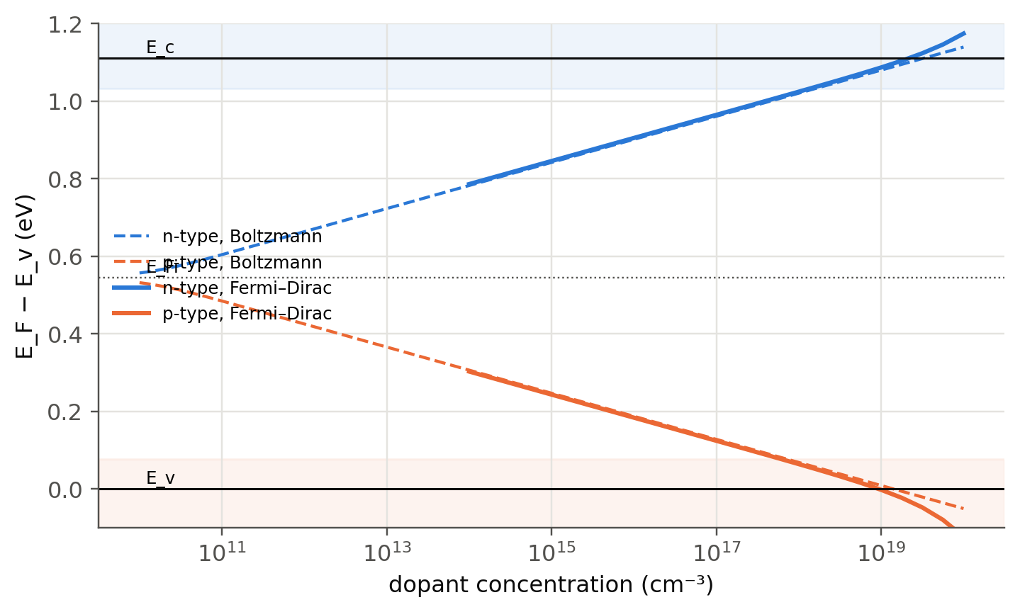
The Fermi level moves away from $E_{Fi}$ by (slides 29–30)
$$
E_{Fn}-E_{Fi}=k_BT\ln\frac{n}{n_i},\qquad E_{Fp}-E_{Fi}=-k_BT\ln\frac{p}{n_i}.
$$
Carriers drift in a field with $v_{de}=\mu_eE_x$, $v_{dh}=\mu_hE_x$, and the conductivity is (slide 18)
$$
\sigma=en\mu_e+ep\mu_h .
$$
The code solves the exact neutrality condition $n+N_a=p+N_d$ with $np=n_i^2$ (`sl.carriers`). It reduces to the formulas above
whenever the net doping is much larger than $n_i$, and it also handles the intermediate cases.
## Doping explorer
```{ojs}
//| echo: false
matD = ({
  Si:   {Eg: 1.11, Nc: 2.8e19, Nv: 1.2e19, ni: 1.0e10, mue: 1450, muh: 490},
  Ge:   {Eg: 0.66, Nc: 1.04e19, Nv: 6.0e18, ni: 2.3e13, mue: 3900, muh: 1900},
  GaAs: {Eg: 1.42, Nc: 4.7e17, Nv: 7.0e18, ni: 2.1e6, mue: 8500, muh: 400}
})
viewof dp = Inputs.form({
  mat: Inputs.select(Object.keys(matD), {value: "Si", label: "material"}),
  lNd: Inputs.range([0, 20], {value: 16, step: 0.05, label: "log₁₀ N_d (cm⁻³), 0 = none"}),
  lNa: Inputs.range([0, 20], {value: 0, step: 0.05, label: "log₁₀ N_a (cm⁻³), 0 = none"}),
  T: Inputs.range([200, 700], {value: 300, step: 5, label: "temperature T (K)"})
})
```
```{ojs}
//| echo: false
dpOut = {
  const m = matD[dp.mat], kT = 8.617333e-5*dp.T;
  const Nc = m.Nc*(dp.T/300)**1.5, Nv = m.Nv*(dp.T/300)**1.5;
  const ni = m.ni*(dp.T/300)**1.5*Math.exp(m.Eg/(2*0.025852) - m.Eg/(2*kT));   // Table 3.1 value at 300 K
  const Nd = dp.lNd > 0 ? 10**dp.lNd : 0, Na = dp.lNa > 0 ? 10**dp.lNa : 0, D = (Nd - Na)/2;
  const r = Math.sqrt(D*D + ni*ni), n = D >= 0 ? D + r : ni*ni/(r - D), p = ni*ni/n;
  const EFi = m.Eg/2 - 0.5*kT*Math.log(Nc/Nv), EF = EFi + kT*Math.log(n/ni);
  const sigma = 1.602e-19*(n*m.mue + p*m.muh);       // S/cm (constant mobilities)
  const type = n > 10*p ? "n-type" : p > 10*n ? "p-type" : "nearly intrinsic";
  return {ni, n, p, EF, EFi, Eg: m.Eg, sigma, type, kT, deg: (m.Eg - EF < 3*kT) || (EF < 3*kT)};
}
Plot.plot({
  width: Math.min(width, 1050), height: 260, x: {domain: [0, 10], axis: null},
  y: {label: "E − E_v (eV)", domain: [-0.25, dpOut.Eg + 0.25], grid: true},
  marks: [
    Plot.rectY([{x1: 0, x2: 10, y1: dpOut.Eg, y2: dpOut.Eg + 0.25}], {x1: "x1", x2: "x2", y1: "y1", y2: "y2", fill: "#2a78d6", fillOpacity: 0.15}),
    Plot.rectY([{x1: 0, x2: 10, y1: -0.25, y2: 0}], {x1: "x1", x2: "x2", y1: "y1", y2: "y2", fill: "#eb6834", fillOpacity: 0.15}),
    Plot.ruleY([0, dpOut.Eg], {stroke: "#0b0b0b", strokeWidth: 2}),
    Plot.ruleY([dpOut.EFi], {stroke: "#52514e", strokeDasharray: "2,3"}),
    Plot.ruleY([dpOut.EF], {stroke: "#4a3aa7", strokeWidth: 2.5, strokeDasharray: "8,4"}),
    Plot.text([{y: dpOut.Eg, t: "E_c"}, {y: 0, t: "E_v"}, {y: dpOut.EFi, t: "E_Fi"}, {y: dpOut.EF, t: "E_F"}],
              {x: 9.9, y: "y", text: "t", textAnchor: "end", dy: -7, fill: "#0b0b0b"}),
    Plot.text([{y: dpOut.Eg + 0.12, t: "conduction band"}, {y: -0.12, t: "valence band"}], {x: 0.2, y: "y", text: "t", textAnchor: "start", fill: "#52514e"})
  ]
})
```
```{ojs}
//| echo: false
html`<div class="result-box"><b>${dpOut.type}</b> · n = <b>${dpOut.n.toExponential(2)}</b> cm⁻³ · p = <b>${dpOut.p.toExponential(2)}</b> cm⁻³ ·
n<sub>i</sub> = ${dpOut.ni.toExponential(2)} cm⁻³<br>
E<sub>F</sub> − E<sub>Fi</sub> = <b>${(dpOut.EF - dpOut.EFi).toFixed(3)} eV</b> · E<sub>c</sub> − E<sub>F</sub> = ${(dpOut.Eg - dpOut.EF).toFixed(3)} eV ·
σ = ${dpOut.sigma.toExponential(2)} S/cm (ρ = ${(1/dpOut.sigma).toExponential(2)} Ω cm, Table 3.1 mobilities)
${dpOut.deg ? html`<br><b>E<sub>F</sub> is within 3k<sub>B</sub>T of a band edge: the material is degenerate, these formulas are no longer accurate.</b>` : ""}</div>`
```
## Worked examples (slides 29–31), recomputed
> **Slides 29–30.** n-type Si with $N_d=10^{16}$ cm$^{-3}$ P. Find $E_{Fn}-E_{Fi}$. Then add $2\times10^{17}$ cm$^{-3}$ B and find
> $E_{Fp}-E_{Fi}$.
> **Slide 31.** Intrinsic conductivity of Si, then $n$, $p$ and $\sigma$ for $N_d=10^{16}$ cm$^{-3}$ with $\mu_e=1200$ cm² V⁻¹ s⁻¹.
```{python}
#| label: tbl-doping-ex
#| tbl-cap: "Slides 29–31 recomputed (n_i = 10¹⁰ cm⁻³, kT = 25.85 meV)."
ni = Si["ni"]
rows = {}
for label, Nd, Na, mue in (("intrinsic Si", 0, 0, Si["mu_e"]),
                           ("Nd = 1e16 (slides 29, 31)", 1e16*CM3, 0, 1200*CM2),
                           ("Nd = 1e16 + Na = 2e17 (slide 30)", 1e16*CM3, 2e17*CM3, Si["mu_e"])):
    n, p = sl.carriers(Nd, Na, ni)
    rows[label] = {"n (cm⁻³)": f"{n/CM3:.3g}", "p (cm⁻³)": f"{p/CM3:.3g}",
                   "E_F − E_Fi (eV)": round(float(sl.fermi_level(n, ni)), 3),
                   "σ (S/cm)": f"{sl.conductivity(n, p, mue, Si['mu_h'])/100:.3g}"}
pd.DataFrame(rows).T
```
The slides give $+0.358$ eV, $-0.434$ eV, $\sigma_i=3.1\times10^{-6}$ Ω⁻¹ cm⁻¹ and $\sigma=1.92$ Ω⁻¹ cm⁻¹. The compensated
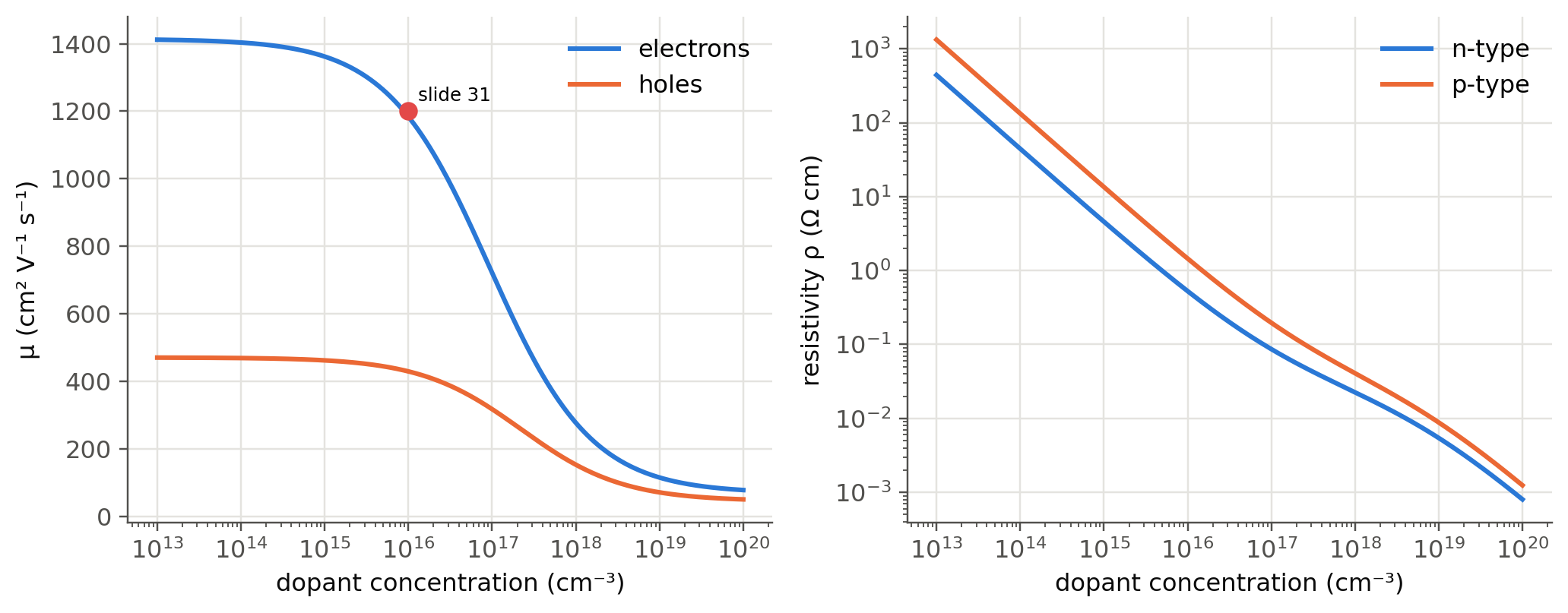
row uses the Table 3.1 hole mobility of 490 cm² V⁻¹ s⁻¹, which is too optimistic at $2\times10^{17}$ cm⁻³ of
ionised impurities (see the mobility section below). Note also that slide 22 is titled "n-Type" and writes $p\approx N_d$:
it describes p-type doping, with $p\approx N_a$.
## Where is the Fermi level?
```{python}
#| label: fig-ef-doping
#| fig-cap: "Fermi level position in Si at 300 K versus net doping. Dashed: Boltzmann formula E_F − E_Fi = ±kT ln(N/n_i). The shaded bands mark where E_F comes within 3kT of a band edge: the material becomes degenerate (slide 28) and the formula overestimates the shift."
N = np.logspace(10, 20, 300)*CM3
kT = sl.kT()
EFi = Si["Eg"]/2 - 0.5*kT*np.log(Si["Nc"]/Si["Nv"])
# exact (Fermi–Dirac) position: solve Nc F1/2((EF−Ec)/kT) − Nv F1/2((Ev−EF)/kT) = Nd − Na
def EF_exact(Nnet):
    f = lambda EF: (Si["Nc"]*sl.fermi_half((EF - Si["Eg"])/kT) - Si["Nv"]*sl.fermi_half(-EF/kT) - Nnet)/abs(Nnet)
    return brentq(f, -0.4, Si["Eg"] + 0.4)
Nn = np.logspace(14, 20, 25)*CM3
fig, ax = plt.subplots()
ax.semilogx(N/CM3, EFi + kT*np.log(sl.carriers(N, 0, Si["ni"])[0]/Si["ni"]), "--", color=sl.PALETTE[0], lw=1.4, label="n-type, Boltzmann")
ax.semilogx(N/CM3, EFi - kT*np.log(sl.carriers(0, N, Si["ni"])[1]/Si["ni"]), "--", color=sl.PALETTE[1], lw=1.4, label="p-type, Boltzmann")
ax.semilogx(Nn/CM3, [EF_exact(x) for x in Nn], color=sl.PALETTE[0], label="n-type, Fermi–Dirac")
ax.semilogx(Nn/CM3, [EF_exact(-x) for x in Nn], color=sl.PALETTE[1], label="p-type, Fermi–Dirac")
ax.axhspan(Si["Eg"] - 3*kT, Si["Eg"] + 0.1, color=sl.PALETTE[0], alpha=0.08); ax.axhspan(-0.1, 3*kT, color=sl.PALETTE[1], alpha=0.08)
for y, t in ((Si["Eg"], "E_c"), (0, "E_v"), (EFi, "E_Fi")):
    ax.axhline(y, color=sl.INK if t != "E_Fi" else sl.INK2, lw=1 if t != "E_Fi" else 0.8, ls="-" if t != "E_Fi" else ":")
    ax.text(1.2e10, y + 0.015, t, fontsize=8)
ax.set(xlabel="dopant concentration (cm⁻³)", ylabel="E_F − E_v (eV)", ylim=(-0.1, 1.2)); ax.legend(fontsize=8, loc="center left")
plt.show()
```
## Mobility depends on doping
The constant mobilities of Table 3.1 hold for lightly doped crystals. Ionised dopants scatter carriers, and the empirical
Caughey–Thomas law describes the drop:
$$
\mu(N)=\mu_\text{min}+\frac{\mu_\text{max}-\mu_\text{min}}{1+(N/N_\text{ref})^\alpha}.
$$
```{python}
#| label: fig-mobility
#| fig-cap: "Si at 300 K: drift mobility (left) and resistivity (right) versus doping (Caughey–Thomas parameters of Masetti/Arora). The slide-31 value μe ≈ 1200 cm²/Vs at 10¹⁶ cm⁻³ is marked."
def mu_ct(N, carrier):
    mmin, mmax, Nref, a = (68.5, 1414, 9.2e16, 0.711) if carrier == "e" else (44.9, 470.5, 2.23e17, 0.719)
    return mmin + (mmax - mmin)/(1 + (N/Nref)**a)      # N in cm^-3, result in cm²/Vs
N = np.logspace(13, 20, 300)
fig, ax = plt.subplots(1, 2, figsize=(9.5, 3.8))
ax[0].semilogx(N, mu_ct(N, "e"), label="electrons"); ax[0].semilogx(N, mu_ct(N, "h"), label="holes")
ax[0].plot(1e16, 1200, "o", color=sl.PALETTE[7], ms=7); ax[0].text(1.3e16, 1230, "slide 31", fontsize=8)
ax[0].set(xlabel="dopant concentration (cm⁻³)", ylabel="μ (cm² V⁻¹ s⁻¹)"); ax[0].legend()
ax[1].loglog(N, 1/(sl.qe*N*mu_ct(N, "e")), label="n-type"); ax[1].loglog(N, 1/(sl.qe*N*mu_ct(N, "h")), label="p-type")
ax[1].set(xlabel="dopant concentration (cm⁻³)", ylabel="resistivity ρ (Ω cm)"); ax[1].legend()
plt.tight_layout(); plt.show()
print(f"μh at 2e17 cm⁻³: {mu_ct(2e17, 'h'):.0f} cm²/Vs (Table 3.1: 490); μe at 1e16: {mu_ct(1e16, 'e'):.0f} cm²/Vs")
```
## Beyond the slides: freeze-out and the intrinsic regime
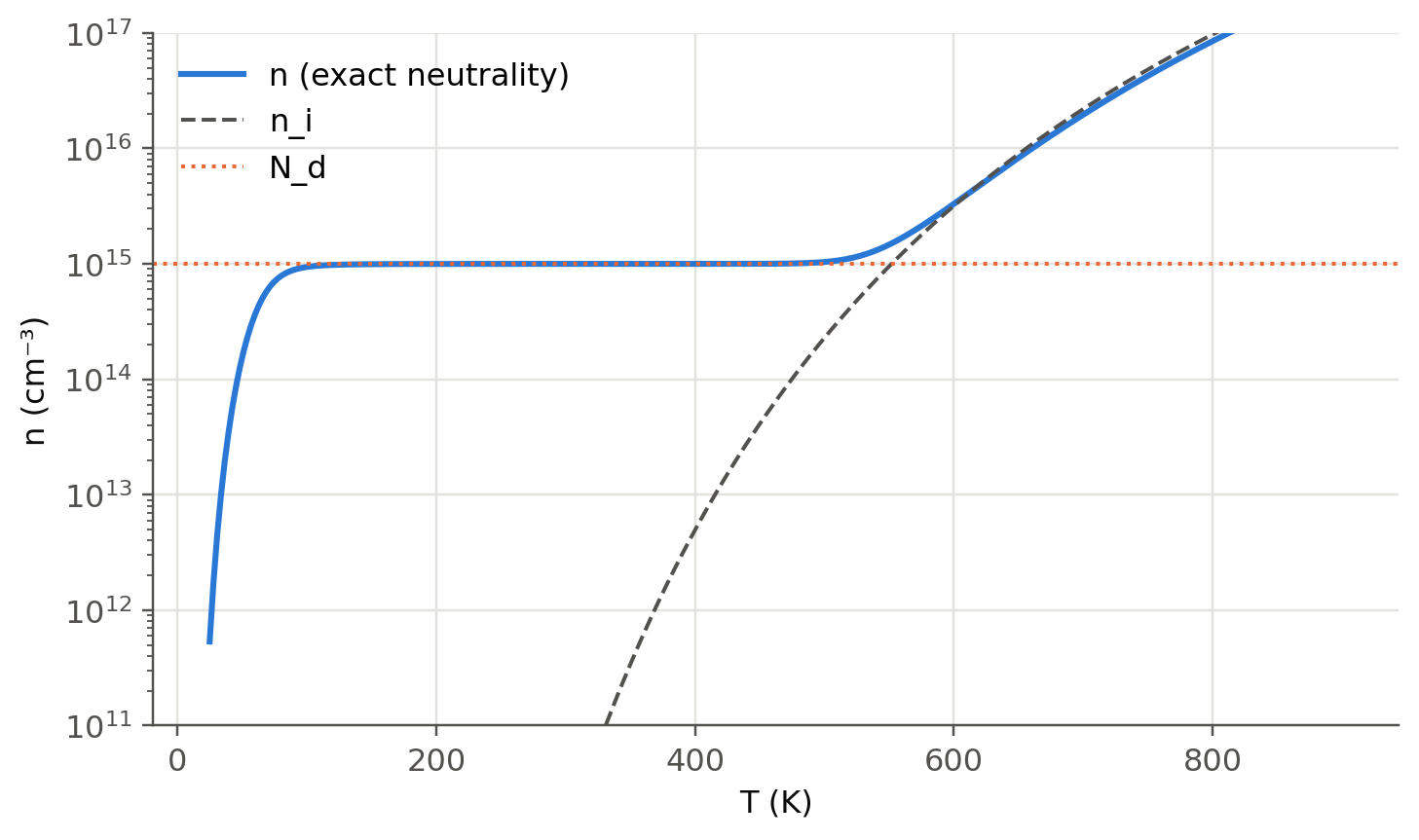
"All donors are ionised" fails at low temperature, where electrons fall back onto the donors (**freeze-out**). It also fails at
high temperature, where $n_i$ overtakes $N_d$. Solving neutrality with the ionised-donor fraction
$N_d^+=N_d/[1+2\exp((E_F-E_d)/k_BT)]$ shows the three regimes of every doped semiconductor:
```{python}
#| label: fig-freezeout
#| fig-cap: "Electron concentration of Si doped with 10¹⁵ cm⁻³ phosphorus (E_c − E_d = 45 meV) versus temperature. Ionisation (freeze-out), extrinsic plateau n ≈ N_d, and intrinsic regime n ≈ n_i. Devices are designed to work on the plateau."
Nd, Ed = 1e15*CM3, 0.045
T = np.linspace(25, 900, 300)
n_out = []
for Tk in T:
    kt = sl.kT(Tk)
    Nc, Nv = Si["Nc"]*(Tk/300)**1.5, Si["Nv"]*(Tk/300)**1.5
    Eg = sl.varshni(Tk, *sl.VARSHNI["Si"]) - sl.varshni(300, *sl.VARSHNI["Si"]) + Si["Eg"]
    def neutral(x):                              # x = (Ec − EF)/kT
        n = Nc*np.exp(-x); p = Nv*np.exp(-(Eg/kt - x)); Ndp = Nd/(1 + 2*np.exp(Ed/kt - x))
        return np.log(n + 1e-300) - np.log(p + Ndp)
    x = brentq(neutral, -5, Eg/kt + 5)
    n_out.append(Nc*np.exp(-x))
n_out = np.array(n_out)
fig, ax = plt.subplots()
ax.semilogy(T, n_out/CM3, label="n (exact neutrality)")
ax.semilogy(T, sl.n_i("Si", T)/CM3, "--", color=sl.INK2, lw=1.3, label="n_i")
ax.axhline(Nd/CM3, color=sl.PALETTE[1], ls=":", lw=1.3, label="N_d")
ax.set(xlabel="T (K)", ylabel="n (cm⁻³)", ylim=(1e11, 1e17)); ax.legend(); plt.show()
```
## Bands tilt in an applied field (slide 32)
A voltage $V$ across a bar of length $L$ adds the potential energy $-eV(x)$ to every electron: the whole band diagram tilts with
slope $eE_x$. Electrons roll "downhill" in the CB, holes "uphill" in the VB, and the Fermi levels at the two contacts differ
by $eV$, exactly the rule of slide 17. A 1 cm Si bar with 1 V applied tilts by 1 eV over 1 cm. The same
picture gives the band bending inside a pn junction (@sec-junction), where the field comes from the space charge.
::: {.callout-tip collapse="true"}
## Going deeper
- **Hall effect.** Combine the drift equations with the Lorentz force to get $R_H=(p\mu_h^2-n\mu_e^2)/[e(p\mu_h+n\mu_e)^2]$. At
which $p/n$ does the Hall coefficient of Si change sign?
- **Minimum conductivity.** Show that $\sigma$ is minimum when $p=n_i\sqrt{\mu_e/\mu_h}$ (slightly p-type), not at intrinsic
doping. Find $\sigma_\text{min}$ for Si and GaAs.
- **Bandgap narrowing.** Heavy doping (> 10¹⁸ cm⁻³) shrinks $E_g$ and raises the effective $n_i$. Look up the Slotboom model
and add it to `EF_exact`. This matters for the emitter of an LED (@sec-spectrum, degenerate junction).
- **Velocity saturation.** $v=\mu E$ breaks down above ~10⁴ V/cm: $v$ saturates near $10^7$ cm/s. Plot $v(E)$ with the
Caughey–Thomas field model.
:::
::: {.callout-note collapse="true"}
## Complements
- Kasap, *Optoelectronics and Photonics*, sec. 3.1; Sze & Ng, ch. 1 (mobility models, freeze-out).
- G. Masetti, M. Severi, S. Solmi, *IEEE Trans. Electron Devices* 30, 764 (1983): doping-dependent mobility in Si.
:::
## Try it yourself
1. A Si wafer has $\rho=1$ Ω cm, n-type. Find $N_d$ with the Caughey–Thomas mobility (use `brentq`).
2. In the explorer, dope Si with $N_d=10^{16}$ cm⁻³ and raise $T$. At what temperature does $p$ reach 10 % of $n$?
3. A GaAs layer must be semi-insulating ($\rho>10^7$ Ω cm). What is the maximum net doping allowed? Why is it easier to obtain
with GaAs than with Si?
4. Repeat the freeze-out figure with B acceptors ($E_a-E_v=45$ meV) and with a deep level at 0.3 eV. What changes?