# LED principle, heterojunctions and materials {#sec-led}
[](https://colab.research.google.com/github/{{< var github_user >}}/{{< var repo >}}/blob/main/{{< var subdir >}}/notebooks/led-principle.ipynb){.colab-link} Run this chapter's code in Google Colab (no installation).
```{python}
#| include: false
import numpy as np
import matplotlib.pyplot as plt
import pandas as pd
import semilib as sl
sl.use_style()
```
*Slides 81–97 (band diagrams under bias, basic LED principle, LED examples, heterojunctions, Np and pP junctions,
quasi-Fermi levels) and 114–119 (LED materials, bandgap versus lattice constant, typical structures, III-nitrides, UV LEDs).*
## Key relations
Forward bias a pn⁺ junction and the barrier drops, so electrons from the n⁺ side are injected into the p side. They recombine
within a diffusion length of the junction and, in a direct-gap semiconductor, emit photons of energy close to the gap (slides
86–87):
$$
h\nu\approx E_g,\qquad \lambda\,[\mu\text{m}]\approx\frac{1.24}{E_g\,[\text{eV}]}.
$$
Under bias the single Fermi level splits into two **quasi-Fermi levels**, $E_{Fn}$ for electrons and $E_{Fp}$ for holes, whose
separation equals $eV$ (slide 87c). The emission colour is set by **bandgap engineering**: alloying binaries such as GaAs and
AlAs or GaN and InN shifts $E_g$ (slides 114–115). The alloy must keep the lattice constant of its substrate, otherwise
dislocations form and kill the radiative efficiency. Vegard's law interpolates the lattice constant,
$a(x)=xa_1+(1-x)a_2$, while the bandgap often bows, $E_g(x)=xE_1+(1-x)E_2-bx(1-x)$.
A **heterojunction** joins two different semiconductors (slides 93–96). Its band edges jump by $\Delta E_c$ and $\Delta E_v$. In a
**double heterostructure** (DH) a thin narrow-gap active layer sits between wide-gap cladding layers. The offsets trap the
injected carriers in the active layer, which raises the recombination rate. The cladding is also transparent to the emitted
photons and has a lower refractive index, so it guides the light. This is the planar waveguide of Chapter 2.
## Alloy colour picker
```{ojs}
//| echo: false
alloys = ({
  "AlxGa1-xAs on GaAs":            {Eg: x => Math.min(1.424 + 1.247*x, 1.900 + 0.125*x + 0.143*x*x), dir: x => 1.424 + 1.247*x <= 1.900 + 0.125*x + 0.143*x*x, a: x => 0.56611*x + 0.56533*(1 - x), sub: 0.56533, lab: "Al fraction x"},
  "GaAs1-yPy (on GaAs/GaP)":       {Eg: y => Math.min(1.424 + 1.150*y + 0.176*y*y, 1.900 + 0.144*y + 0.211*y*y), dir: y => 1.424 + 1.150*y + 0.176*y*y <= 1.900 + 0.144*y + 0.211*y*y, a: y => 0.54505*y + 0.56533*(1 - y), sub: 0.56533, lab: "P fraction y"},
  "(AlxGa1-x)0.5In0.5P on GaAs":   {Eg: x => Math.min(1.91 + 0.61*x, 2.19 + 0.085*x), dir: x => 1.91 + 0.61*x <= 2.19 + 0.085*x, a: x => 0.5653, sub: 0.56533, lab: "Al fraction x"},
  "In(1-x)Ga(x)As(y)P(1-y) on InP": {Eg: y => 1.35 - 0.72*y + 0.12*y*y, dir: y => true, a: y => 0.58687, sub: 0.58687, lab: "As fraction y (lattice-matched, x ≈ 0.47y)"},
  "InxGa1-xN on GaN":              {Eg: x => 3.42*(1 - x) + 0.77*x - 1.43*x*(1 - x), dir: x => true, a: x => 0.3545*x + 0.3189*(1 - x), sub: 0.3189, lab: "In fraction x"},
  "AlxGa1-xN on GaN":              {Eg: x => 3.42*(1 - x) + 6.05*x - 1.0*x*(1 - x), dir: x => true, a: x => 0.3112*x + 0.3189*(1 - x), sub: 0.3189, lab: "Al fraction x"}
})
viewof al = Inputs.form({
  name: Inputs.select(Object.keys(alloys), {value: "InxGa1-xN on GaN", label: "alloy"}),
  x: Inputs.range([0, 1], {value: 0.15, step: 0.005, label: "composition"})
})
```
```{ojs}
//| echo: false
alOut = {
  const A = alloys[al.name], data = [];
  for (let i = 0; i <= 200; i++) { const x = i/200; data.push({x, Eg: A.Eg(x), lam: 1239.84/A.Eg(x), direct: A.dir(x)}); }
  const Eg = A.Eg(al.x), lam = 1239.84/Eg, a = A.a(al.x);
  // Bruton's wavelength to RGB (indicative)
  const rgb = (w) => { let r = 0, g = 0, b = 0;
    if (w >= 380 && w < 440) { r = (440 - w)/60; b = 1; } else if (w < 490 && w >= 440) { g = (w - 440)/50; b = 1; }
    else if (w < 510 && w >= 490) { g = 1; b = (510 - w)/20; } else if (w < 580 && w >= 510) { r = (w - 510)/70; g = 1; }
    else if (w < 645 && w >= 580) { r = 1; g = (645 - w)/65; } else if (w <= 780 && w >= 645) { r = 1; }
    else return "rgb(90,90,90)";
    const f = w < 420 ? 0.3 + 0.7*(w - 380)/40 : w > 700 ? 0.3 + 0.7*(780 - w)/80 : 1;
    return `rgb(${[r, g, b].map(c => Math.round(255*(f*c)**0.8)).join(",")})`; };
  return {data, Eg, lam, a, mis: (a - A.sub)/A.sub*100, color: rgb(lam), direct: A.dir(al.x), lab: A.lab};
}
Plot.plot({
  width: Math.min(width, 1050), height: 300, x: {label: alOut.lab, domain: [0, 1]},
  y: {label: "emission wavelength hc/E_g (nm)", grid: true},
  marks: [
    Plot.line(alOut.data, {x: "x", y: "lam", stroke: "#2a78d6", strokeWidth: 2}),
    Plot.dot(alOut.data.filter(d => !d.direct), {x: "x", y: "lam", r: 2, fill: "#e34948"}),
    Plot.dot([{x: al.x, y: alOut.lam}], {x: "x", y: "y", r: 9, fill: alOut.color, stroke: "#0b0b0b", strokeWidth: 1.5}),
    Plot.ruleY([380, 780], {stroke: "#52514e", strokeDasharray: "3,3"})
  ]
})
```
```{ojs}
//| echo: false
html`<div class="result-box" style="display:flex;gap:1rem;align-items:center"><div style="width:56px;height:56px;border-radius:8px;background:${alOut.color};border:1px solid #888"></div>
<div>E<sub>g</sub> = <b>${alOut.Eg.toFixed(3)} eV</b> · λ ≈ <b>${alOut.lam.toFixed(0)} nm</b> (${alOut.lam < 380 ? "ultraviolet" : alOut.lam > 780 ? "infrared" : "visible"}) ·
${alOut.direct ? "direct gap" : html`<b style="color:#e34948">indirect gap: poor emitter</b>`}<br>
lattice constant a = ${alOut.a.toFixed(4)} nm · mismatch to substrate = <b>${alOut.mis.toFixed(2)} %</b>
${Math.abs(alOut.mis) > 1 ? " (strained: only thin layers possible)" : ""}</div></div>`
```
The red dots mark compositions with an **indirect** gap (AlGaAs above $x\approx0.45$, GaAsP above $y\approx0.45$): the material
still absorbs, but emits poorly (@sec-direct). Note the InGaN curve: a modest In fraction (15–30 %) covers violet to green. This
is why the blue LED (Nobel Prize 2014) was a materials breakthrough. Very high In content is hard to grow because of the 11 %
lattice mismatch with GaN.
## Bandgap versus lattice constant (slide 115)
```{python}
#| label: fig-eg-a
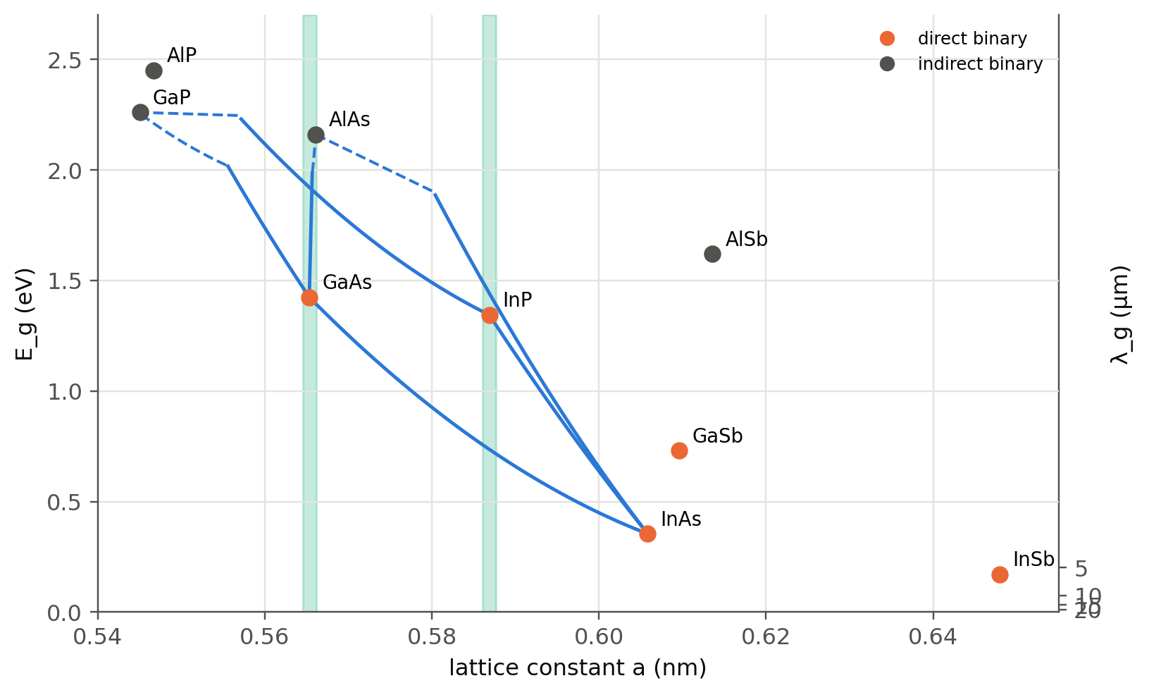
#| fig-cap: "Bandgap versus lattice constant of III–V compounds (slide 115). Lines are ternary alloys; dashed segments are indirect. The vertical bands are the GaAs and InP lattice constants: AlGaAs is lattice-matched to GaAs for any x, and InGaAsP covers 0.75–1.35 eV (1.65–0.92 µm) on InP, the telecom range."
L = sl.LATTICE
binaries = {"GaAs": 1.424, "AlAs": 2.16, "InAs": 0.354, "GaP": 2.26, "InP": 1.344, "AlP": 2.45, "GaSb": 0.73, "InSb": 0.17, "AlSb": 1.62}
direct = {"GaAs", "InAs", "InP", "GaSb", "InSb"}
fig, ax = plt.subplots(figsize=(8, 5))
x = np.linspace(0, 1, 101)
# (direct Γ gap, indirect gap or None) as functions of the fraction x of the FIRST binary
lines = {("AlAs", "GaAs"): (lambda x: 1.424 + 1.247*x, lambda x: 1.900 + 0.125*x + 0.143*x**2),
         ("GaP", "GaAs"):  (lambda x: 1.424 + 1.150*x + 0.176*x**2, lambda x: 1.900 + 0.144*x + 0.211*x**2),
         ("GaAs", "InAs"): (lambda x: 0.354*(1 - x) + 1.424*x - 0.477*x*(1 - x), None),
         ("InP", "InAs"):  (lambda x: 0.354*(1 - x) + 1.344*x - 0.10*x*(1 - x), None),
         ("GaP", "InP"):   (lambda x: 1.344*(1 - x) + 2.78*x - 0.65*x*(1 - x), lambda x: 2.21 + 0.05*x),
         ("AlAs", "InAs"): (lambda x: 0.354*(1 - x) + 3.0*x - 0.70*x*(1 - x), lambda x: 1.43*(1 - x) + 2.16*x)}
for (b1, b2), (fG, fX) in lines.items():
    a = sl.vegard(L[b1], L[b2], x)
    EG = fG(x); EX = fX(x) if fX else np.full_like(x, np.inf)
    Eg = np.minimum(EG, EX)
    ax.plot(a, np.where(EG <= EX, Eg, np.nan), color=sl.PALETTE[0], lw=1.6)
    ax.plot(a, np.where(EG > EX, Eg, np.nan), color=sl.PALETTE[0], lw=1.3, ls="--")
for b, Eg in binaries.items():
    ax.plot(L[b], Eg, "o", ms=7, color=sl.PALETTE[1] if b in direct else sl.INK2, zorder=5)
    ax.annotate(b, (L[b], Eg), textcoords="offset points", xytext=(6, 4), fontsize=9)
for b in ("GaAs", "InP"): ax.axvspan(L[b] - 0.0008, L[b] + 0.0008, color=sl.PALETTE[2], alpha=0.25)
sec = ax.secondary_yaxis("right", functions=(lambda E: 1.24/np.maximum(E, 0.05), lambda l: 1.24/np.maximum(l, 0.05)))
sec.set_ylabel("λ_g (µm)")
ax.set(xlabel="lattice constant a (nm)", ylabel="E_g (eV)", xlim=(0.54, 0.655), ylim=(0, 2.7))
ax.plot([], [], "o", color=sl.PALETTE[1], label="direct binary"); ax.plot([], [], "o", color=sl.INK2, label="indirect binary")
ax.legend(fontsize=8, loc="upper right"); plt.show()
```
The ternary bowing parameters are representative textbook values (Vurgaftman *et al.*, 2001). For quantitative design use the
full direct and indirect gap parameters of that review.
## LED materials and colours (slide 114)
```{python}
#| label: tbl-led-materials
#| tbl-cap: "Representative LED materials, their emission wavelengths and substrates (slides 114–119). The colour column uses the photopic sensitivity V(λ) of @sec-efficiency."
leds = [("GaN/InGaN MQW", "sapphire, SiC, Si", 1239.84/405, "violet / UV-A"),
        ("InGaN MQW", "sapphire, SiC", 1239.84/460, "blue"),
        ("InGaN MQW", "sapphire, SiC", 1239.84/525, "green"),
        ("AlGaInP", "GaAs", 1239.84/590, "amber"),
        ("AlGaInP", "GaAs", 1239.84/625, "red"),
        ("GaAs₀.₆P₀.₄", "GaAs", 1239.84/650, "red (early LEDs)"),
        ("Al₀.₃Ga₀.₇As", "GaAs", 1239.84/820, "near IR"),
        ("GaAs", "GaAs", 1239.84/870, "IR remote controls"),
        ("InGaAsP", "InP", 1239.84/1310, "fiber, O band"),
        ("InGaAsP", "InP", 1239.84/1550, "fiber, C band"),
        ("AlGaN", "sapphire, AlN", 1239.84/280, "UV-C, disinfection")]
pd.DataFrame([{"active material": m, "substrate": s, "E_g (eV)": round(E, 2), "λ (nm)": round(1239.84/E),
               "V(λ)": f"{float(sl.V_photopic(1239.84/E*1e-9)):.3g}", "use": u} for m, s, E, u in leds])
```
## Heterojunctions: carrier and photon confinement (slides 93–97)
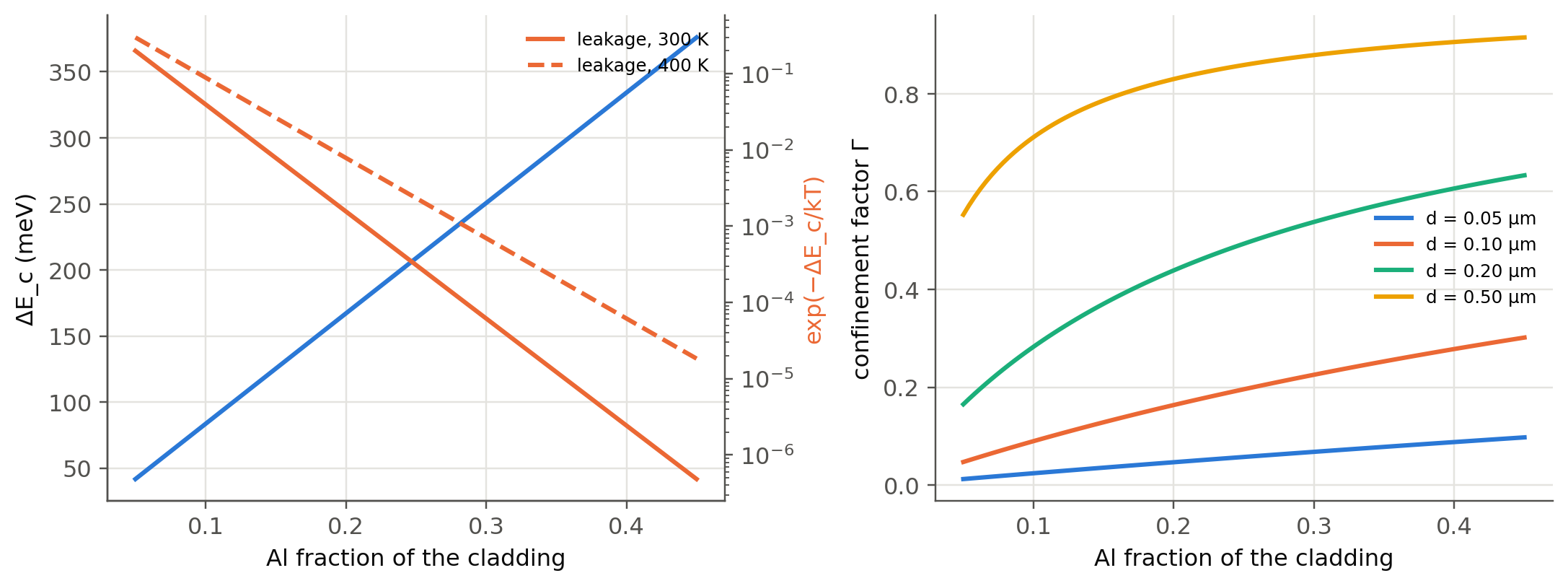
Two numbers show why every modern LED is a heterostructure. The fraction of injected electrons that spill over a barrier
$\Delta E_c$ is about $\exp(-\Delta E_c/k_BT)$. The fraction of the guided light that overlaps the active layer is the
**optical confinement factor** $\Gamma$ of the slab waveguide formed by the index step:
```{python}
#| label: fig-dh
#| fig-cap: "AlGaAs/GaAs double heterostructure (λ ≈ 870 nm). Left: band offset ΔEc = 0.67 ΔEg and the Boltzmann leakage factor exp(−ΔEc/kT) versus cladding Al fraction. Right: confinement factor Γ of the fundamental TE mode of the active layer (slab waveguide, Botez approximation Γ ≈ D²/(2 + D²) with D = k₀d(n₁² − n₂²)^½)."
x = np.linspace(0.05, 0.45, 100)
dEc = 0.67*1.247*x
nGaAs = 3.59; n_cl = 3.59 - 0.53*x                      # index at 870 nm decreases with Al (approx.)
fig, ax = plt.subplots(1, 2, figsize=(10, 3.8))
ax[0].plot(x, dEc*1e3, label="ΔE_c (meV)")
a2 = ax[0].twinx(); a2.semilogy(x, np.exp(-dEc/sl.kT(300)), color=sl.PALETTE[1], label="leakage, 300 K")
a2.semilogy(x, np.exp(-dEc/sl.kT(400)), "--", color=sl.PALETTE[1], label="leakage, 400 K")
a2.set_ylabel("exp(−ΔE_c/kT)", color=sl.PALETTE[1]); a2.spines["right"].set_visible(True); a2.grid(False); a2.legend(fontsize=8)
ax[0].set(xlabel="Al fraction of the cladding", ylabel="ΔE_c (meV)")
for d in (0.05e-6, 0.1e-6, 0.2e-6, 0.5e-6):
    V = 2*np.pi*d/870e-9*np.sqrt(nGaAs**2 - n_cl**2)   # Botez normalised thickness k0 d NA
    ax[1].plot(x, V**2/(2 + V**2), label=f"d = {d*1e6:.2f} µm")
ax[1].set(xlabel="Al fraction of the cladding", ylabel="confinement factor Γ"); ax[1].legend(fontsize=8)
plt.tight_layout(); plt.show()
```
With $x=0.3$ cladding, $\Delta E_c\approx0.25$ eV and the leakage is below $10^{-4}$. A 0.1–0.2 µm active layer confines
20–60 % of the guided light. Edge-emitting LEDs (@sec-drive) and laser diodes (Ch. 4) exploit both effects. The Np and pP
heterojunction band diagrams of slides 95–96 follow the same rule as homojunctions: flat $E_F$ at equilibrium, bands bent by the
space charge, plus the offsets $\Delta E_c$ and $\Delta E_v$ at the interface.
### Simulating a double heterostructure {#sec-dh-sim}
The drift–diffusion simulator of @sec-ddsim showed why a homojunction is a poor LED. The injected electrons spread over a
diffusion length of several µm, so their density stays low, and the radiative rate per electron, $BN_a$, is fixed by the
doping. The panel below adds the band offsets. A p-GaAs active layer of thickness $d$ sits between a p-Al$_x$Ga$_{1-x}$As
cladding ($N_a=3\times10^{18}$ cm⁻³) and an n-Al$_x$Ga$_{1-x}$As cladding ($N_d=3\times10^{17}$ cm⁻³), with
$\Delta E_g=1.247x$ eV split 67:33 between $\Delta E_c$ and $\Delta E_v$. The **reference** is the same structure with
$x=0$: identical doping, no offsets, so it is a homojunction. Both use $B=10^{-10}$ cm³ s⁻¹, $C_n=C_p=10^{-30}$ cm⁶ s⁻¹ and the
SRH lifetime below, everywhere.
LEDs are compared at equal **current**, not equal voltage, so the slider sets the current density $J$. The simulator picks the
nearest computed bias point for each structure.
```{ojs}
//| echo: false
import {PNDiode} from "./pn_led_sim.js"
```
```{ojs}
//| echo: false
viewof dhp = Inputs.form({
  x: Inputs.range([0, 0.45], {value: 0.3, step: 0.01, label: "cladding Al fraction x"}),
  d: Inputs.range([10, 1000], {value: 100, step: 10, label: "active layer thickness d (nm)"}),
  lNa: Inputs.range([15, 19], {value: 17, step: 0.1, label: "log₁₀ active-layer doping N_a (cm⁻³)"}),
  ltau: Inputs.range([-9, -6], {value: -7, step: 0.1, label: "log₁₀ SRH lifetime τ_n = τ_p (s)"})
})
```
```{ojs}
//| echo: false
dhStep = 0.025
dhVmax = 1.5
dhOff = ({dEg: 1.247 * dhp.x, dEc: 0.67 * 1.247 * dhp.x, dEv: 0.33 * 1.247 * dhp.x})
// two voltage sweeps (heterostructure and reference), computed in chunks; a change of any input restarts them
dhSim = {
  const mk = (x) => new PNDiode({
    Na: 3e18, Nd: 3e17, tau_n: 10 ** dhp.ltau, tau_p: 10 ** dhp.ltau, mesh: [2e-7, 3e-5, 1.1, 1e-5],
    dh: {d: dhp.d * 1e-7, dEc: 0.67 * 1.247 * x, dEv: 0.33 * 1.247 * x, Nact: -(10 ** dhp.lNa)}
  });
  const keys = ["DH", "ref"], devs = {DH: mk(dhp.x), ref: mk(0)}, res = {DH: [], ref: []}, fail = {DH: null, ref: null}, u = {};
  yield Promises.delay(150, {devs, res, fail, done: false});
  for (const k of keys) {
    const r = devs[k].solve(devs[k].initialGuess(), 0, {maxit: 400});
    if (r.ok) u[k] = r.u; else fail[k] = 0;
  }
  const nV = Math.round(dhVmax / dhStep);
  for (let s = 1; s <= nV; s++) {
    for (const k of keys) {
      if (fail[k] !== null) continue;
      const r = devs[k].solve(u[k], s * dhStep);
      if (!r.ok) { fail[k] = s * dhStep; continue; }
      u[k] = r.u;
      res[k].push(devs[k].analyse(u[k], s * dhStep));
    }
    if (s % 5 === 0 && s < nV) yield {devs, res, fail, done: false};
  }
  yield {devs, res, fail, done: true};
}
```
```{ojs}
//| echo: false
// IQE, light from the active layer and recombination outside it, along each sweep
dhRows = {
  const out = {};
  for (const k of ["DH", "ref"]) out[k] = dhSim.res[k].filter((a) => a.J > 0).map((a, i) => {
    const rad = a.rad_p + a.rad_n + a.rad_scl, act = a.rad_act + a.srh_act + a.aug_act;
    const pr = a.profile, dev = dhSim.devs[k];
    let nmax = 0;
    for (let j = dev.iL; j <= dev.iR; j++) nmax = Math.max(nmax, Math.min(pr.n[j], pr.p[j]));
    return {k, V: a.V, J: a.J, IQE: rad / a.J, radAct: rad > 0 ? a.rad_act / rad : NaN, outside: 1 - act / a.J, nmin: nmax, a};
  });
  return out;
}
viewof dhJ = Inputs.range([-2, 3], {value: 1.5, step: 0.1, label: "log₁₀ current density J (A/cm²)"})
viewof dhXw = Inputs.range([0.1, 10], {value: 2, step: 0.1, label: "x window ± (µm)"})
```
```{ojs}
//| echo: false
dhSel = {
  const pick = (rows) => rows.length ? rows.reduce((b, r) => Math.abs(Math.log10(r.J) - dhJ) < Math.abs(Math.log10(b.J) - dhJ) ? r : b) : null;
  return {DH: pick(dhRows.DH), ref: pick(dhRows.ref)};
}
dhCols = ({rad: "#1f9e6a", srh: "#eb6834", aug: "#7b4fd0", n: "#2a78d6", p: "#d63a5a", ref: "#8a8986"})
dhPow = (d) => { const e = Math.log10(d); return Number.isInteger(e) ? "10" + String(e).split("").map((c) => "⁻⁰¹²³⁴⁵⁶⁷⁸⁹"["-0123456789".indexOf(c)]).join("") : ""; }
{
  const s = dhSim, pct = (v) => Number.isFinite(v) ? (100 * v).toFixed(1) + " %" : "–";
  const status = !s.done ? html`<i>simulating… ${s.res.DH.length ? `reached ${s.res.DH[s.res.DH.length - 1].V.toFixed(2)} V` : "equilibrium"}</i><br>`
    : ["DH", "ref"].filter((k) => s.fail[k] !== null).map((k) => html`<b>${k}: Newton did not converge at ${s.fail[k].toFixed(3)} V; sweep stopped there.</b><br>`);
  const line = (k, name) => {
    const r = dhSel[k];
    if (!r) return "";
    return html`<b>${name}</b>: J = ${r.J.toExponential(2)} A/cm² at V = ${r.V.toFixed(3)} V · IQE = <b>${pct(r.IQE)}</b> ·
      light from the active layer ${pct(r.radAct)} · recombination outside it ${pct(r.outside)} ·
      min(n, p) in the layer up to ${r.nmin.toExponential(1)} cm⁻³<br>`;
  };
  return html`<div class="result-box">${status}
    ΔE<sub>g</sub> = ${(1000 * dhOff.dEg).toFixed(0)} meV: ΔE<sub>c</sub> = ${(1000 * dhOff.dEc).toFixed(0)} meV,
    ΔE<sub>v</sub> = ${(1000 * dhOff.dEv).toFixed(0)} meV (ΔE<sub>c</sub> = ${(dhOff.dEc / 0.02585).toFixed(1)} k<sub>B</sub>T)<br>
    ${line("DH", "heterostructure")}${line("ref", "reference (x = 0)")}</div>`;
}
```
```{ojs}
//| echo: false
Plot.plot({
  width: Math.min(width, 1050), height: 280,
  x: {type: "log", label: "current density J (A/cm²)", domain: [1e-2, 1e3], tickFormat: dhPow},
  y: {label: "IQE = Jrad/J (%)", domain: [0, 100], grid: true},
  title: "Internal quantum efficiency at equal current (vertical line: selected J)",
  color: {legend: true, domain: ["heterostructure", "reference (x = 0)"], range: [dhCols.rad, dhCols.ref]},
  marks: [
    Plot.ruleX([10 ** dhJ], {stroke: "currentColor", strokeOpacity: 0.35}),
    Plot.line(dhRows.DH.filter((d) => d.J >= 1e-2 && d.J <= 1e3), {x: "J", y: (d) => 100 * d.IQE, stroke: () => "heterostructure", strokeWidth: 2.4}),
    Plot.line(dhRows.ref.filter((d) => d.J >= 1e-2 && d.J <= 1e3), {x: "J", y: (d) => 100 * d.IQE, stroke: () => "reference (x = 0)", strokeWidth: 2, strokeDasharray: "6,3"})
  ]
})
```
```{ojs}
//| echo: false
// spatial profiles of both structures at the selected current
dhProf = {
  const conv = (k) => {
    const r = dhSel[k];
    if (!r) return [];
    const pr = r.a.profile, dev = dhSim.devs[k], rows = [];
    for (let i = 0; i < pr.x.length; i++) {
      const x = pr.x[i] * 1e4;
      if (Math.abs(x) > dhXw) continue;
      rows.push({x, Ec: -dev.Vt * (pr.psi[i] + pr.thn[i]) + dev.Eg / 2, Ev: -dev.Vt * (pr.psi[i] - pr.thp[i]) - dev.Eg / 2,
                 Fn: -dev.Vt * pr.fn[i], Fp: -dev.Vt * pr.fp[i], n: pr.n[i], p: pr.p[i],
                 rad: pr.Rrad[i], srh: pr.Rsrh[i], aug: pr.Raug[i]});
    }
    return rows;
  };
  return {DH: conv("DH"), ref: conv("ref"), act: [{x1: -dhp.d * 5e-4, x2: dhp.d * 5e-4}]};
}
dhX = ({label: "x (µm)   ← p cladding | active | n cladding →", domain: [-dhXw, dhXw]})
dhAct = Plot.rect(dhProf.act, {x1: "x1", x2: "x2", fill: dhCols.rad, fillOpacity: 0.08})
dhSel.DH ? Plot.plot({
  width: Math.min(width, 1050), height: 250, x: dhX, y: {label: "energy (eV)", grid: true},
  title: `Heterostructure bands and quasi-Fermi levels at J = ${dhSel.DH.J.toExponential(1)} A/cm² (shaded: active layer)`,
  color: {legend: true, domain: ["Ec, Ev", "EFn", "EFp"], range: ["currentColor", dhCols.n, dhCols.p]},
  marks: [
    dhAct,
    Plot.line(dhProf.DH, {x: "x", y: "Ec", stroke: () => "Ec, Ev", strokeWidth: 2}),
    Plot.line(dhProf.DH, {x: "x", y: "Ev", stroke: () => "Ec, Ev", strokeWidth: 2}),
    Plot.line(dhProf.DH, {x: "x", y: "Fn", stroke: () => "EFn", strokeDasharray: "6,3", strokeWidth: 1.8}),
    Plot.line(dhProf.DH, {x: "x", y: "Fp", stroke: () => "EFp", strokeDasharray: "6,3", strokeWidth: 1.8})
  ]
}) : html``
```
```{ojs}
//| echo: false
dhSel.DH ? Plot.plot({
  width: Math.min(width, 1050), height: 250, x: dhX, y: {type: "log", label: "concentration (cm⁻³)", grid: true, tickFormat: dhPow},
  title: "Carriers at the same current: heterostructure (solid) and reference (dashed)",
  color: {legend: true, domain: ["n", "p"], range: [dhCols.n, dhCols.p]},
  marks: [
    dhAct,
    Plot.line(dhProf.ref, {x: "x", y: "n", stroke: () => "n", strokeDasharray: "4,3", strokeOpacity: 0.6}),
    Plot.line(dhProf.ref, {x: "x", y: "p", stroke: () => "p", strokeDasharray: "4,3", strokeOpacity: 0.6}),
    Plot.line(dhProf.DH, {x: "x", y: "n", stroke: () => "n", strokeWidth: 2}),
    Plot.line(dhProf.DH, {x: "x", y: "p", stroke: () => "p", strokeWidth: 2})
  ]
}) : html``
```
```{ojs}
//| echo: false
dhSel.DH ? (() => {
  const all = [...dhProf.DH, ...dhProf.ref];
  const rmax = Math.max(...all.map((d) => Math.max(d.rad, d.srh, d.aug))), floor = rmax / 1e6;
  const keep = (rows, k) => rows.filter((d) => d[k] > floor);
  return Plot.plot({
    width: Math.min(width, 1050), height: 300, x: dhX,
    y: {type: "log", label: "R(x) (cm⁻³ s⁻¹)", grid: true, domain: [floor, rmax * 2], tickFormat: dhPow,
        ticks: d3.range(Math.ceil(Math.log10(floor)), Math.floor(Math.log10(rmax * 2)) + 1).map((e) => 10 ** e)},
    title: "Recombination at the same current (green area: B·n·p in the heterostructure; grey: B·n·p in the reference)",
    color: {legend: true, domain: ["radiative", "SRH", "Auger", "radiative, reference"], range: [dhCols.rad, dhCols.srh, dhCols.aug, dhCols.ref]},
    marks: [
      dhAct,
      Plot.areaY(keep(dhProf.DH, "rad"), {x: "x", y1: floor, y2: "rad", fill: dhCols.rad, fillOpacity: 0.18}),
      Plot.line(keep(dhProf.DH, "rad"), {x: "x", y: "rad", stroke: () => "radiative", strokeWidth: 2.2}),
      Plot.line(keep(dhProf.DH, "srh"), {x: "x", y: "srh", stroke: () => "SRH", strokeWidth: 2, strokeDasharray: "6,3"}),
      Plot.line(keep(dhProf.DH, "aug"), {x: "x", y: "aug", stroke: () => "Auger", strokeWidth: 2, strokeDasharray: "2,3"}),
      Plot.line(keep(dhProf.ref, "rad"), {x: "x", y: "rad", stroke: () => "radiative, reference", strokeWidth: 2})
    ]
  });
})() : html``
```
What to look for, with the default structure ($x=0.3$, $d=100$ nm, $N_a=10^{17}$ cm⁻³, $\tau=100$ ns):
1. **Carrier confinement.** In the band diagram, $\Delta E_c$ stops the electrons at the p-cladding side and $\Delta E_v$ stops the
holes at the n-cladding side. Both carriers pile up in the active layer, and essentially all the light comes from it. In the
carrier plot, at 30 A/cm² both $n$ and $p$ in the layer reach about $4\times10^{17}$ cm⁻³. That is several hundred times the
electron density injected into the p side of the reference, where the electrons spread over several µm.
2. **The IQE grows with current.** Once $n\approx p\gg N_a$ in the layer, the radiative rate goes as $Bn^2$ while SRH goes as
$n/2\tau$, so $\eta_\text{IQE}\approx 2B\tau n/(1+2B\tau n)$ rises with the injection. In the reference both rates are linear
in the minority density and the IQE barely changes with $J$. The heterostructure wins above a few A/cm².
3. **At low current the heterostructure is worse.** With $n\approx p$ the whole lightly doped layer behaves like the SCL of a
homojunction, where SRH is strongest. Raise the active doping to $10^{18}$ cm⁻³ and watch the low-current IQE recover.
4. **Thickness.** A thinner layer gives a higher density at the same current, so the IQE rises earlier. Below about 20 nm the
electron levels are quantised: this is a quantum well (@sec-qw), which this classical model does not describe.
5. **Barrier height.** Lower $x$ toward 0.05. With $\Delta E_c$ only a few $k_BT$, electrons spill into the p cladding and the
recombination outside the layer grows.
6. **Lifetime.** With $\tau=10$ ns the heterostructure needs about 50 A/cm² to beat the reference. The quality of the active
layer and of its interfaces matters as much as the band offsets.
The model leaves out the largest practical advantage of the heterostructure: the claddings are **transparent** to photons of
energy $E_g(\text{GaAs})$. In a homojunction most photons are generated a few µm deep in GaAs, which absorbs them
($1/\alpha\approx1$ µm near the gap), whereas here they cross the claddings unattenuated. Other simplifications: abrupt offsets
spread over one 2 nm mesh cell (no thermionic emission), no interface recombination, and the same masses, mobilities and
permittivity in GaAs and AlGaAs.
::: {.callout-tip collapse="true"}
## Going deeper
- **Anderson's rule** predicts $\Delta E_c=\chi_1-\chi_2$. Use the electron affinities of Table 3.1 for GaAs/AlAs and compare with
the measured 65:35 split of $\Delta E_g$. Why does the rule fail?
- **Critical thickness.** A strained layer can grow without dislocations only up to the Matthews–Blakeslee thickness. Estimate it
for In$_{0.2}$Ga$_{0.8}$N on GaN (mismatch ~2.2 %).
- **The green gap.** Plot the EQE of commercial LEDs against wavelength: it drops between 530 and 600 nm, where neither InGaN nor
AlGaInP works well. Find the physical reasons for each side.
- **Polarisation fields.** Wurtzite InGaN quantum wells carry MV/cm piezoelectric fields that tilt the well, shift the emission
to the red and separate electrons from holes (quantum-confined Stark effect). Connect with @sec-qw.
:::
::: {.callout-note collapse="true"}
## Complements
- Kasap, *Optoelectronics and Photonics*, sec. 3.8–3.12; E. F. Schubert, *Light-Emitting Diodes*, 3rd ed. (2018), ch. 4, 12–16.
- I. Vurgaftman, J. R. Meyer, L. R. Ram-Mohan, "Band parameters for III–V compound semiconductors and their alloys",
*J. Appl. Phys.* 89, 5815 (2001).
- H. Kroemer, "Quasi-electric fields and band offsets", *Rev. Mod. Phys.* 73, 783 (2001) (slide 93); S. Nakamura, Nobel lecture
(2014) (slide 117).
:::
## Try it yourself
1. Which In fraction of InGaN emits at 450 nm? At 530 nm? What lattice mismatch to GaN does each imply?
2. Find the composition of In$_{1-x}$Ga$_x$As$_y$P$_{1-y}$ on InP that emits at 1310 nm.
3. Why is AlGaAs with $x>0.45$ used as a cladding but never as an active layer?
4. Using `sl.vegard`, find the Ga fraction of In$_{1-x}$Ga$_x$As lattice-matched to InP, and its emission wavelength.