# Capacitance and the small-signal model {#sec-smallsignal}
[](https://colab.research.google.com/github/{{< var github_user >}}/{{< var repo >}}/blob/main/{{< var subdir >}}/notebooks/smallsignal.ipynb){.colab-link} Run this chapter's code in Google Colab (no installation).
```{python}
#| include: false
import numpy as np
import matplotlib.pyplot as plt
import pandas as pd
import semilib as sl
sl.use_style()
CM3, CM2 = sl.CM3, sl.CM2
```
*Slides 70–74: depletion capacitance, dynamic resistance, diffusion capacitance (long and short diodes), small-signal
equivalent circuit.*
## Key relations
The SCL stores charge $\pm Q$ separated by $W$, like a parallel-plate capacitor whose gap changes with the voltage. Its
incremental capacitance is the **depletion capacitance** (slides 70 and 74):
$$
C_\text{dep}=\left|\frac{dQ}{dV}\right|=\frac{\varepsilon A}{W}=\frac{A}{(V_o-V)^{1/2}}\left[\frac{e\varepsilon N_aN_d}{2(N_a+N_d)}\right]^{1/2}
\ \xrightarrow{\ p^+n\ }\ A\left[\frac{e\varepsilon N_d}{2(V_o-V)}\right]^{1/2}.
$$
Under forward bias the injected minority charge $Q=\tau_hI$ also changes with $V$. This gives a **dynamic resistance** and a
**diffusion capacitance** (slides 71–73):
$$
r_d=\frac{dV}{dI}=\frac{\eta V_\text{th}}{I},\qquad
C_\text{diff}=\frac{\tau_hI}{2V_\text{th}}=\frac{\tau_h}{2r_d}\ \text{(long diode, ac)},\qquad
C_\text{diff}=\frac{\tau_tI}{V_\text{th}}\ \text{(short diode, } \tau_t=\ell_n^2/2D_h),
$$
with $V_\text{th}=k_BT/e$. The small-signal equivalent circuit is a series resistance $r_s$ followed by $r_d$, $C_\text{diff}$
and $C_\text{dep}$ in parallel (slide 71c). $C_\text{dep}$ dominates under reverse bias (photodiodes, varactors) and
$C_\text{diff}$ under forward bias (LEDs).
## C–V explorer
The dashed grey curves are the three junctions of slide 70(b). Your junction is the solid line.
```{ojs}
//| echo: false
viewof cv = Inputs.form({
  lNa: Inputs.range([14, 19], {value: 16.7, step: 0.05, label: "log₁₀ N_a (cm⁻³)"}),
  lNd: Inputs.range([14, 19], {value: 15.0, step: 0.05, label: "log₁₀ N_d (cm⁻³)"}),
  er: Inputs.range([10, 16], {value: 11.8, step: 0.1, label: "ε_r (Si 11.8, GaAs 13)"}),
  ni: Inputs.select(new Map([["Si (1e10)", 1e10], ["GaAs (2.1e6)", 2.1e6], ["Ge (2.3e13)", 2.3e13]]), {value: 1e10, label: "n_i"})
})
```
```{ojs}
//| echo: false
cvOut = {
  const q = 1.602176634e-19, kT = 0.025852, e0 = 8.8541878e-12;
  const curve = (Na, Nd, er, ni, label) => {
    const Vo = kT*Math.log(Na*Nd/ni**2), out = [];
    for (let V = -10; V < Math.min(0.7, Vo - 0.05); V += 0.02) {
      const W = Math.sqrt(2*er*e0*(Na + Nd)*(Vo - V)/(q*Na*Nd));
      out.push({V, C: er*e0*1e-6/W*1e12, label});    // pF per mm²
    }
    return out;
  };
  const ref = [[5e22, 5e22, "5e16 / 5e16"], [5e22, 5e20, "5e16 / 5e14"], [5e20, 5e20, "5e14 / 5e14"]]
    .flatMap(([a, d, l]) => curve(a, d, 11.8, 1e16, l));
  const mine = curve(10**cv.lNa*1e6, 10**cv.lNd*1e6, cv.er, cv.ni*1e6, "yours");
  return {ref, mine, Vo: kT*Math.log(10**(cv.lNa + cv.lNd)/cv.ni**2)};
}
Plot.plot({
  width: Math.min(width, 1050), height: 330, x: {label: "V (V)", domain: [-10, 0.8]},
  y: {type: "log", label: "C_dep (pF mm⁻²)", grid: true, domain: [5, 2000]},
  marks: [
    Plot.line(cvOut.ref, {x: "V", y: "C", z: "label", stroke: "#52514e", strokeWidth: 1.2, strokeDasharray: "5,4"}),
    Plot.text(cvOut.ref.filter(d => Math.abs(d.V + 8) < 0.011), {x: "V", y: "C", text: "label", dy: -8, fill: "#52514e", fontSize: 10}),
    Plot.line(cvOut.mine, {x: "V", y: "C", stroke: "#2a78d6", strokeWidth: 2.5}),
    Plot.tip(cvOut.mine, Plot.pointerX({x: "V", y: "C", title: d => `V = ${d.V.toFixed(2)} V\nC = ${d.C.toFixed(1)} pF/mm²`}))
  ]
})
```
```{ojs}
//| echo: false
html`<div class="result-box">V<sub>o</sub> = ${cvOut.Vo.toFixed(3)} V · C<sub>dep</sub>(0) = <b>${cvOut.mine.find(d => d.V >= 0)?.C.toFixed(1)} pF/mm²</b> ·
C<sub>dep</sub>(−5 V) = ${cvOut.mine.find(d => d.V >= -5)?.C.toFixed(1)} pF/mm²</div>`
```
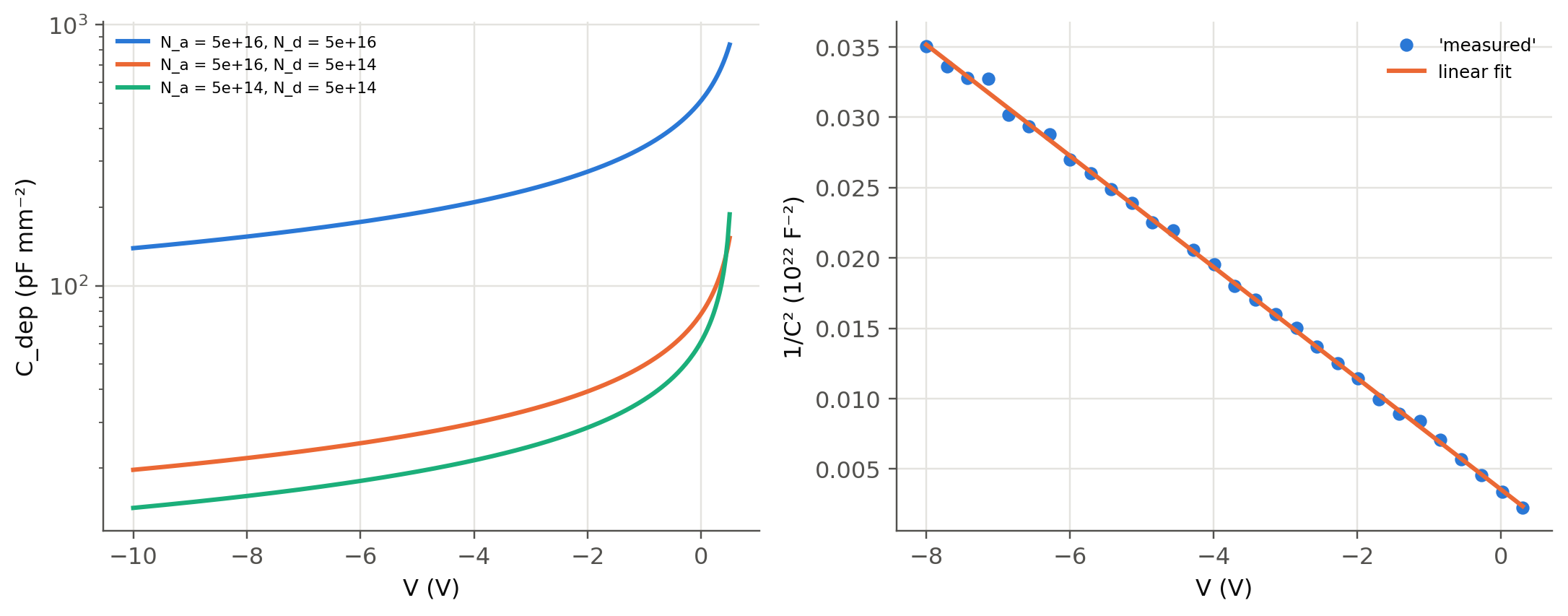
The capacitance is set by the **lightly doped side**: the 5×10¹⁶/5×10¹⁴ junction is almost identical to the 5×10¹⁴/5×10¹⁴
one. The curve ends near $V_o$, where the depletion approximation breaks down (and $C_\text{diff}$ takes over).
## Slide 70(b) and Mott–Schottky profiling
```{python}
#| label: fig-cv
#| fig-cap: "Left: C_dep per mm² for the three Si junctions of slide 70(b). Right: 1/C² versus V is a straight line whose slope gives the doping of the light side and whose intercept gives V_o (Mott–Schottky plot), here applied to a synthetic 'measurement' with 1 % noise."
fig, ax = plt.subplots(1, 2, figsize=(10, 4))
V = np.linspace(-10, 0.5, 300)
p = sl.MATERIALS["Si"]
for Na, Nd in ((5e16, 5e16), (5e16, 5e14), (5e14, 5e14)):
    Vo = sl.built_in_voltage(Na*CM3, Nd*CM3, p["ni"])
    Vv = V[V < Vo - 0.05]
    ax[0].semilogy(Vv, sl.c_dep(1e-6, Na*CM3, Nd*CM3, p["eps_r"], Vo, Vv)*1e12, label=f"N_a = {Na:.0e}, N_d = {Nd:.0e}")
ax[0].set(xlabel="V (V)", ylabel="C_dep (pF mm⁻²)"); ax[0].legend(fontsize=7)

# synthetic measurement on a p⁺n junction, then fit
rng = np.random.default_rng(1)
Na, Nd, A = 1e19*CM3, 3e15*CM3, 1e-6
Vo = sl.built_in_voltage(Na, Nd, p["ni"])
Vm = np.linspace(-8, 0.3, 30)
Cm = sl.c_dep(A, Na, Nd, p["eps_r"], Vo, Vm)*(1 + 0.01*rng.standard_normal(Vm.size))
slope, icpt = np.polyfit(Vm, 1/Cm**2, 1)
Nd_fit = -2/(sl.qe*p["eps_r"]*sl.eps0*A**2*slope)
ax[1].plot(Vm, 1/Cm**2/1e22, "o", ms=5, label="'measured'")
ax[1].plot(Vm, np.polyval([slope, icpt], Vm)/1e22, label="linear fit")
ax[1].set(xlabel="V (V)", ylabel="1/C² (10²² F⁻²)"); ax[1].legend(fontsize=8)
plt.tight_layout(); plt.show()
print(f"true N_d = {Nd/CM3:.2e} cm⁻³, fitted N_d = {Nd_fit/CM3:.2e} cm⁻³;  true V_o = {Vo:.3f} V, fitted V_o = {-icpt/slope:.3f} V")
```
For a p⁺n junction $1/C_\text{dep}^2=2(V_o-V)/(e\varepsilon N_dA^2)$, so $N_d=-2/(e\varepsilon A^2\,d(1/C^2)/dV)$. Applied
point by point, with $W=\varepsilon A/C$ as the depth, the same formula gives the **doping profile** $N_d(W)$. This is the
standard C–V characterisation of LED and photodiode wafers.
## Forward bias: $r_d$ and $C_\text{diff}$ of an LED
```{python}
#| label: tbl-smallsignal
#| tbl-cap: "Small-signal elements of the GaAs diode of slides 75–80 (A = 1 mm², τ = 50 ns, long diode) at several forward currents. At LED operating currents C_diff exceeds C_dep by orders of magnitude, and r_d C_diff = τ/2 does not depend on the current."
p = sl.MATERIALS["GaAs"]
Na = Nd = 1e23; A = 1e-6; tau = 50e-9
Vo = sl.built_in_voltage(Na, Nd, p["ni"])
gaas = dict(A=A, Na=Na, Nd=Nd, mat="GaAs", B=2e-16, mu_e=5000*CM2, mu_h=250*CM2)
rows = {}
for V in (0.8, 1.0, 1.05, 1.1):
    d = sl.diode_currents(V, **gaas)
    I = float(d["I"]); dI = float(sl.diode_currents(V + 1e-4, **gaas)["I"]) - I
    rd = 1e-4/dI
    Cd = sl.c_diff(float(d["I_diff"]), tau)            # only the diffusion part stores minority charge
    Cj = sl.c_dep(A, Na, Nd, p["eps_r"], Vo, V)
    rows[f"V = {V} V"] = {"I (mA)": I*1e3, "r_d (Ω)": rd, "C_dep (pF)": Cj*1e12, "C_diff (pF)": Cd*1e12,
                          "r_d(C_dep + C_diff) (ns)": rd*(Cj + Cd)*1e9}
pd.DataFrame(rows).T.map(lambda v: f"{v:.3g}")
```
At low bias the recombination current has no stored minority charge, $\eta=2$, and the RC product is set by $C_\text{dep}$. At
LED operating currents $r_dC_\text{diff}\to\tau/2$: the diode cannot respond faster than its minority carrier lifetime. This
is the electrical side of the LED modulation bandwidth of @sec-drive, $f_{3\text{dB}}\propto1/\tau$.
## Impedance of the equivalent circuit
```{python}
#| label: fig-impedance
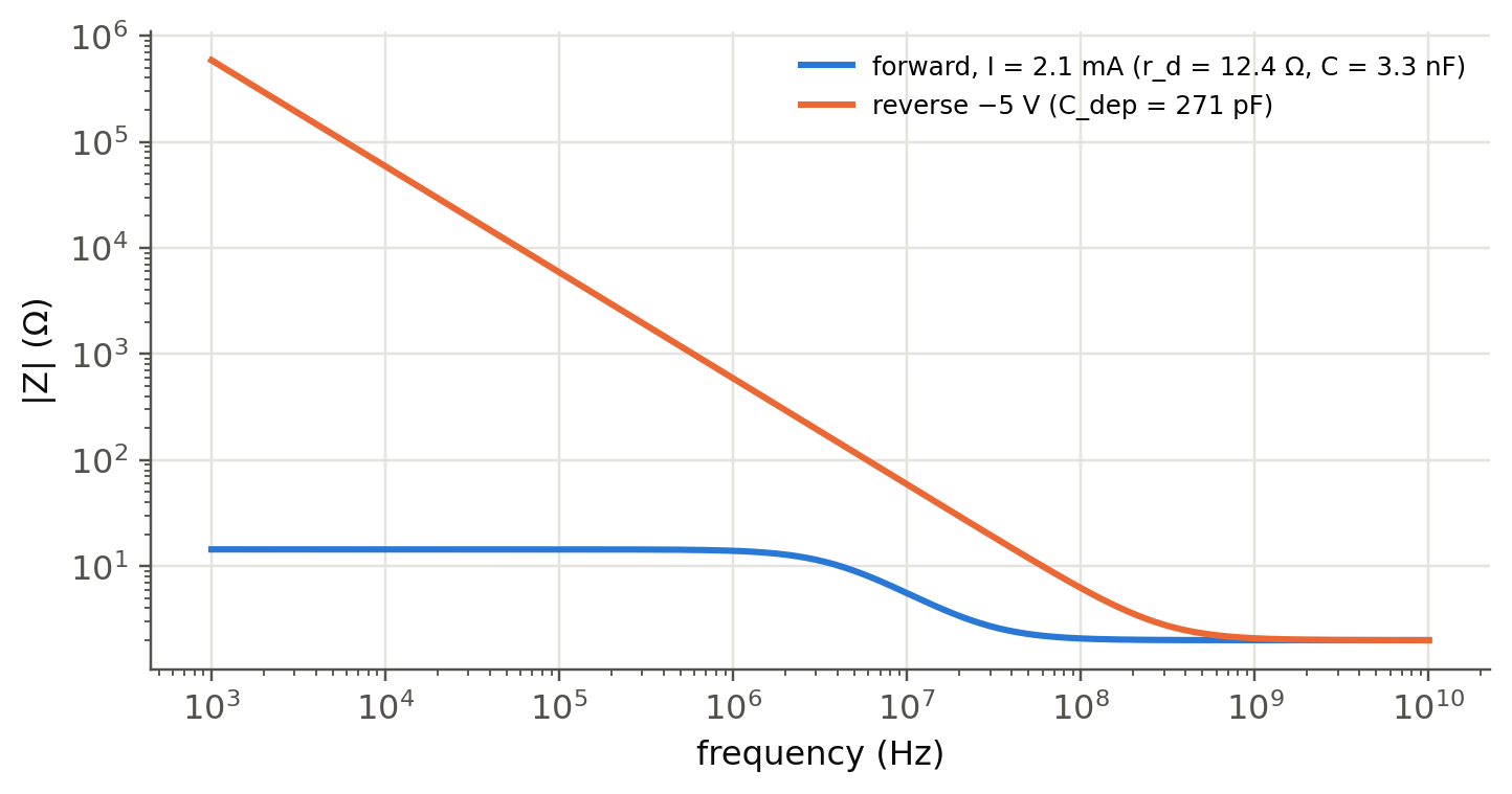
#| fig-cap: "Magnitude of the small-signal impedance of the GaAs diode at 1.05 V (r_s = 2 Ω) and at −5 V reverse bias. Forward: r_d ∥ C_diff rolls off at f = 1/(2π r_d C) ≈ 1/(πτ). Reverse: a pure depletion capacitance."
f = np.logspace(3, 10, 400); w = 2*np.pi*f; rs = 2.0
d = sl.diode_currents(1.05, **gaas); I = float(d["I_diff"] + d["I_rec"])
rd = sl.r_d(I); Cf = sl.c_diff(float(d["I_diff"]), tau) + sl.c_dep(A, Na, Nd, p["eps_r"], Vo, 1.05)
Cr = sl.c_dep(A, Na, Nd, p["eps_r"], Vo, -5)
Zf = rs + rd/(1 + 1j*w*rd*Cf); Zr = rs + 1/(1j*w*Cr)
fig, ax = plt.subplots(figsize=(7.5, 3.6))
ax.loglog(f, abs(Zf), label=f"forward, I = {I*1e3:.1f} mA (r_d = {rd:.1f} Ω, C = {Cf*1e9:.1f} nF)")
ax.loglog(f, abs(Zr), label=f"reverse −5 V (C_dep = {Cr*1e12:.0f} pF)")
ax.set(xlabel="frequency (Hz)", ylabel="|Z| (Ω)"); ax.legend(fontsize=8); plt.show()
```
::: {.callout-tip collapse="true"}
## Going deeper
- **Varactors.** A hyperabrupt doping profile $N_d\propto x^{-3/2}$ gives $C\propto(V_o-V)^{-2}$ and a resonance frequency
linear in voltage. Simulate a VCO tuning curve.
- **Why $\tau/2$ and not $\tau$?** Solve the time-dependent diffusion equation with a small sinusoidal injection: the
admittance of a long diode is $Y=(1/r_d)\sqrt{1+j\omega\tau_h}$. Expand for $\omega\tau\ll1$ to recover $C_\text{diff}=\tau_h/2r_d$.
- **Doping profiles.** Apply the point-by-point Mott–Schottky formula to a synthetic junction with a graded doping and check that
you recover the profile.
- **Photodiode speed.** In Chapter 5 the RC time of $C_\text{dep}$ with a 50 Ω load competes with the transit time across $W$.
Find the reverse bias that minimises the total response time of a Si pin diode.
:::
::: {.callout-note collapse="true"}
## Complements
- Kasap, *Optoelectronics and Photonics*, sec. 3.7; Sze & Ng, ch. 2 (C–V, admittance of a long diode).
- D. K. Schroder, *Semiconductor Material and Device Characterization*, ch. 2 (C–V doping profiling).
:::
## Try it yourself
1. A Si p⁺n photodiode of 1 mm² with $N_d=10^{14}$ cm⁻³ is reverse biased at 10 V. Find $C_\text{dep}$ and the RC limit with 50 Ω.
2. An LED driven at 20 mA has $\tau=5$ ns. Compute $r_d$ and $C_\text{diff}$. Which driver output impedance keeps the electrical
bandwidth above the optical one?
3. Show that $C_\text{dep}$ of a p⁺n junction depends on $N_d$ only through $\sqrt{N_d}$. How much must the doping change to halve it?