Dielectric Waveguides and Optical Fibers

An interactive companion to Chapter 2 — Optoelectronics

Preface

“The introduction of optical fiber systems will revolutionize the communications network. The low-transmission loss and the large bandwidth capability of the fiber systems allow signals to be transmitted for establishing communications contacts over large distances with few or no provisions of intermediate amplification.” — Charles K. Kao, 1982 (Nobel Prize in Physics, 2009)

This companion follows the slides of Chapter 2 — Dielectric Waveguides and Optical Fibers section by section. The slides tell the story; this book lets you compute it. Every figure is produced by a few lines of Python that you can unfold (“Show the Python”), copy, and modify. Most chapters also have live panels (sliders, marked with a blue bar on the left) that recompute directly in your browser. They need no Python installation.

How the book is organised

Chapter	Slides	What you can play with
Planar waveguides	7–39	graphical mode solver, TIR phase, mode fields, dispersion diagram, \(v_g(\omega)\)
Step-index fibers	40–64	exact LP-mode solver, \(b\)–\(V\) chart, 2-D mode patterns, MFD, fiber designer
Dispersion	65–95	Sellmeier glasses, \(D_m\), \(D_w\), zero-dispersion engineering, PMD random walk, compensation
Graded-index fibers	122–134	ray tracing in a GRIN core, optimum profile \(\gamma\), GRIN rod lens
Attenuation & bending	135–162	loss spectrum builder, Rayleigh limit, bend-loss fitting
Bit rate & capacity	96–121	Nyquist/Shannon, Gaussian pulse broadening, a full IM/DD link simulator with eye diagrams
WDM, couplers & nonlinearity	174–194	ITU grid, couplers, star couplers, four-wave-mixing product map, SPM chirp, SBS
Special fibers & FBGs	195–230	Bragg fibers, coupled-mode FBG spectra, strain/temperature sensing
Fiber sensors	231–311	OTDR trace simulator, Raman DTS, Brillouin, Fabry–Perot, Sagnac gyroscope
Projects & new ideas	—	suggestions to extend the course

Each chapter ends with “Try it yourself” exercises. Where a slide contains a worked example, the companion recomputes it and gives the number, so you can check your hand calculation.

NoteNotation used throughout

\(n_1\) core index, \(n_2\) cladding index, \(a\) core radius (fiber) or half-thickness (slab), \(\Delta=(n_1^2-n_2^2)/2n_1^2\approx (n_1-n_2)/n_1\), \(\mathrm{NA}=\sqrt{n_1^2-n_2^2}\), \(V=\frac{2\pi a}{\lambda}\mathrm{NA}\), \(b=(n_\text{eff}^2-n_2^2)/(n_1^2-n_2^2)\). Python uses SI units. Dispersion is quoted in ps nm\(^{-1}\) km\(^{-1}\).

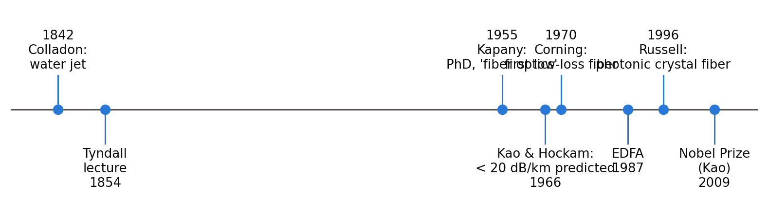
A bit of history (slides 1–5)

import matplotlib.pyplot as plt
import fiberlib as fl
fl.use_style()

events = [(1842, "Colladon:\nwater jet"), (1854, "Tyndall\nlecture"),
          (1955, "Kapany:\nPhD, 'fiber optics'"), (1966, "Kao & Hockam:\n< 20 dB/km predicted"),
          (1970, "Corning:\nfirst low-loss fiber"), (1987, "EDFA"),
          (1996, "Russell:\nphotonic crystal fiber"), (2009, "Nobel Prize\n(Kao)")]
fig, ax = plt.subplots(figsize=(9, 2.4))
ax.axhline(0, color=fl.INK2, lw=1)
for i, (y, txt) in enumerate(events):
    up = 1 if i % 2 == 0 else -1
    ax.plot([y, y], [0, 0.55 * up], color=fl.PALETTE[0], lw=1)
    ax.plot(y, 0, "o", ms=6, color=fl.PALETTE[0])
    ax.text(y, 0.62 * up, f"{y}\n{txt}" if up > 0 else f"{txt}\n{y}",
            ha="center", va="bottom" if up > 0 else "top", fontsize=8.5, color=fl.INK)
ax.set_ylim(-1.6, 1.6); ax.set_xlim(1830, 2020)
ax.axis("off")
plt.show()

Figure 1: Some milestones of light guiding mentioned in the slides.

The time axis is not linear in “interest”: it took more than a century to go from Colladon’s water jet to a usable glass fiber. The breakthrough was materials purity (Kao’s prediction that intrinsic glass losses could fall below 20 dB/km), not a new idea about guiding. The chapter Attenuation & bending shows why: today’s 0.15–0.2 dB/km sit close to the Rayleigh limit of silica.

Running the code without installing anything

Every chapter starts with an Open in Colab button that opens its code as a notebook in Google Colab. Colab is free and runs in the browser; you only need a Google account. The interactive ipywidgets explorers are here:

Open in Colab

To keep your changes, use File → Save a copy in Drive in Colab.

Using the code

All functions live in a small, readable module, fiberlib.py (~400 lines), which you can import from your own notebooks:

import fiberlib as fl
fl.LP_all(V=5)                 # list of guided LP modes (l, m, b)
fl.D_material(1.55e-6)         # material dispersion of silica [s/m^2]

See the appendix Running the notebooks for installation, and for how to turn every chapter into a Jupyter notebook.