# Attenuation and bending loss {#sec-attenuation}
[](https://colab.research.google.com/github/{{< var github_user >}}/{{< var repo >}}/blob/main/{{< var subdir >}}/notebooks/attenuation.ipynb){.colab-link} Run this chapter's code in Google Colab (no installation).
```{python}
#| include: false
import numpy as np
import matplotlib.pyplot as plt
import fiberlib as fl
fl.use_style()
c0 = fl.c0
```
*Slides 135–162.* Attenuation = absorption + scattering. Power decays exponentially,
$P_\text{out}=P_\text{in}e^{-\alpha L}$, and engineers quote it in dB:
$$
\alpha_\text{dB}=\frac{10}{L}\log_{10}\frac{P_\text{in}}{P_\text{out}}=4.34\,\alpha .
$$
## The loss spectrum of silica (slides 136–142)
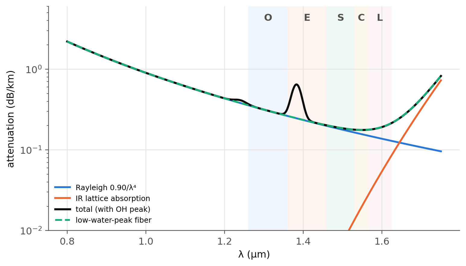
Four contributions shape the classic "V" curve:
- **Rayleigh scattering** $\alpha_R=A_R/\lambda^4$ from frozen-in density fluctuations,
- **infrared (lattice, Reststrahlen) absorption** $\alpha_{FIR}=A\,e^{-B/\lambda}$ with
$A=7.81\times10^{11}$ dB/km and $B=48.48$ µm,
- **ultraviolet (Urbach) tail** from electronic transitions, negligible in the IR,
- **OH⁻ overtones**, chiefly at 1383 nm (and 1240 nm). "Low-water-peak" fibers (G.652.D) remove them and
open the E-band.
```{python}
#| label: fig-loss
#| fig-cap: "Model loss spectrum of a silica SMF and its components. The minimum near 1550 nm (≈ 0.18 dB/km) is set by Rayleigh scattering on one side and lattice absorption on the other."
lam = np.linspace(0.8, 1.75, 600) * 1e-6
um = lam * 1e6
tot = fl.attenuation_model(lam, AR=0.90, OH_peak=0.4)
fig, ax = plt.subplots(figsize=(8, 4.4))
ax.semilogy(um, 0.90 / um**4, color=fl.PALETTE[0], label="Rayleigh 0.90/λ⁴")
ax.semilogy(um, 7.81e11 * np.exp(-48.48 / um), color=fl.PALETTE[1], label="IR lattice absorption")
ax.semilogy(um, tot, color=fl.INK, lw=2.2, label="total (with OH peak)")
ax.semilogy(um, fl.attenuation_model(lam, AR=0.90, OH_peak=0.0), "--", color=fl.PALETTE[2], label="low-water-peak fiber")
bands = {"O": (1260, 1360), "E": (1360, 1460), "S": (1460, 1530), "C": (1530, 1565), "L": (1565, 1625)}
for k, (b, (l1, l2)) in enumerate(bands.items()):
    ax.axvspan(l1 / 1e3, l2 / 1e3, color=fl.PALETTE[k % 8], alpha=0.07, lw=0)
    ax.text((l1 + l2) / 2e3, 4, b, ha="center", fontweight="bold", color=fl.INK2)
ax.set_ylim(0.01, 6); ax.set_xlabel("λ (µm)"); ax.set_ylabel("attenuation (dB/km)")
ax.legend(fontsize=8, loc="lower left"); plt.show()
i = np.argmin(tot); print(f"Minimum: {tot[i]:.3f} dB/km at {um[i]*1e3:.0f} nm")
```
### Build your own fiber loss, live
```{ojs}
//| echo: false
viewof att = Inputs.form({
  AR: Inputs.range([0.5, 1.5], {value: 0.90, step: 0.01, label: "A_R (dB km⁻¹ µm⁴)"}),
  OH: Inputs.range([0, 3], {value: 0.4, step: 0.05, label: "OH peak at 1383 nm (dB/km)"}),
  L:  Inputs.range([1, 200], {value: 80, step: 1, label: "link length (km)"}),
  P0: Inputs.range([-10, 20], {value: 3, step: 0.5, label: "launch power (dBm)"})
})
```
```{ojs}
//| echo: false
attModel = l => att.AR / l**4 + 7.81e11*Math.exp(-48.48/l) + att.OH*Math.exp(-0.5*((l-1.383)/0.012)**2) + 0.08*att.OH*Math.exp(-0.5*((l-1.24)/0.015)**2)
attData = d3.range(0.8, 1.75, 0.002).map(l => ({l: l*1000, a: attModel(l)}))
Plot.plot({
  width: Math.min(width, 1050), height: 320, y: {type: "log", domain: [0.05, 6], label: "attenuation (dB/km)", grid: true}, x: {label: "λ (nm)"},
  marks: [Plot.line(attData, {x: "l", y: "a", stroke: "#2a78d6", strokeWidth: 2.5}),
          Plot.ruleX([1310, 1550], {stroke: "#b9b8b2", strokeDasharray: "4,3"}),
          Plot.tip(attData, Plot.pointerX({x: "l", y: "a", title: d => `${d.l.toFixed(0)} nm\n${d.a.toFixed(3)} dB/km`}))]
})
```
```{ojs}
//| echo: false
html`<div class="result-box">${[0.85, 1.31, 1.383, 1.55, 1.625].map(l =>
  `λ = ${(l*1000).toFixed(0)} nm: α = ${attModel(l).toFixed(3)} dB/km → after ${att.L} km: P = ${(att.P0 - attModel(l)*att.L).toFixed(1)} dBm`).join("<br>")}</div>`
```
## Rayleigh scattering: the ultimate limit (slides 138–139)
$$
\alpha_R\approx\frac{8\pi^3}{3\lambda^4}(n^2-1)^2\beta_T k_BT_f
$$
where $\beta_T$ is the isothermal compressibility and $T_f$ the fictive temperature.
```{python}
aR = fl.rayleigh_alpha(1.55e-6, 1.4446, 7e-11, 1730 + 273)
print(f"Slide 139: α_R = {aR:.3e} m⁻¹ = {aR*1e3:.3e} km⁻¹ → {4.34*aR*1e3:.3f} dB/km at 1.55 µm")
for lam in [0.85, 1.31, 1.55]:
    print(f"   at {lam} µm: {4.34e3*fl.rayleigh_alpha(lam*1e-6, 1.4446, 7e-11, 2003):.3f} dB/km")
```
Lowering $T_f$ (annealing, or alkali-doped "pure-silica-core" fibers) reduces scattering. Ultra-low-loss
fibers reach about 0.14–0.15 dB/km, and hollow-core fibers have now gone below 0.1 dB/km (@sec-special).
### Example (slides 145–147)
$A_R$ depends on the doping: $A_R\approx0.63+2.06\,\mathrm{NA}$ dB km$^{-1}$ µm$^4$ for GeO$_2$-doped step-index fibers.
```{python}
NA_ = 0.14
aFIR = 7.81e11 * np.exp(-48.48 / 1.55)
for lam in [1.55, 1.31]:
    r1 = 0.90 / lam**4
    AR = 0.63 + 2.06 * NA_
    r2 = AR / lam**4
    extra = aFIR if lam == 1.55 else 0
    print(f"λ = {lam} µm: α_FIR = {extra:.3f}, rule of thumb {r1:.3f} → total {r1+extra:.3f};  "
          f"A_R(NA) = {AR:.3f} → {r2:.3f} → total {r2+extra:.3f} dB/km")
```
## Bending loss (slides 148–162)
When the fiber is bent, the part of the mode beyond a critical radius would have to travel faster than light
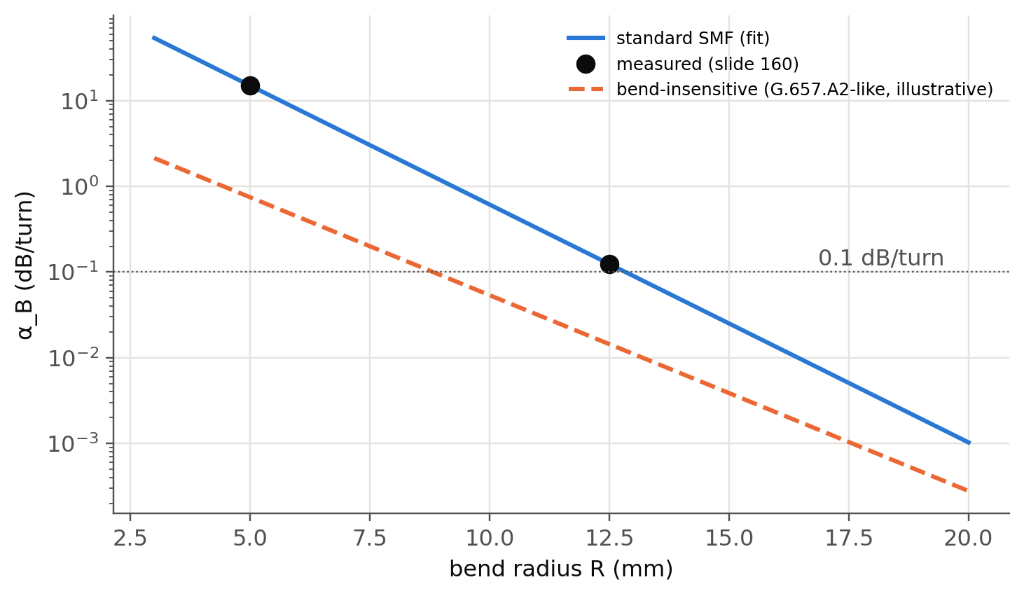
to keep the wavefront plane, so it radiates (slide 152). Empirically,
$$
\alpha_B = A\,e^{-R/R_c}.
$$
### Example: fit two measurements (slide 160)
```{python}
#| label: fig-bend
#| fig-cap: "Bend loss of a standard SMF at 1550 nm from the two-point fit of slide 160, compared with typical values for bend-insensitive G.657 fibers (trench-assisted, slides 153–154)."
R1, a1, R2, a2 = 12.5, 0.124, 5.0, 15.0
Rc = (R1 - R2) / np.log(a2 / a1)
A = a2 * np.exp(R2 / Rc)
print(f"R_c = {Rc:.2f} mm, A = {A:.0f} dB/turn, α_B(10 mm) = {A*np.exp(-10/Rc):.2f} dB/turn")
R = np.linspace(3, 20, 200)
fig, ax = plt.subplots()
ax.semilogy(R, A * np.exp(-R / Rc), label="standard SMF (fit)")
ax.semilogy([R1, R2], [a1, a2], "o", color=fl.INK, ms=8, label="measured (slide 160)")
ax.semilogy(R, 0.2 * np.exp(-(R - 7.5) / 1.9), "--", label="bend-insensitive (G.657.A2-like, illustrative)")
ax.axhline(0.1, color=fl.INK2, lw=0.8, ls=":"); ax.text(19.5, 0.12, "0.1 dB/turn", ha="right", color=fl.INK2)
ax.set_xlabel("bend radius R (mm)"); ax.set_ylabel("α_B (dB/turn)"); ax.legend(fontsize=8)
plt.show()
```
### MAC number (slides 156–158)
$N_\text{MAC}=\mathrm{MFD}/\lambda_c$. Bend loss grows exponentially with it. A large MFD (good for splicing and
for low nonlinearity) and a short cut-off both make the fiber more bend-sensitive.
```{python}
for name, mfd, lc in [("G.652 SMF", 9.2, 1.26), ("G.657 (smaller MFD)", 8.6, 1.26), ("large-MFD fiber", 10.5, 1.26)]:
    print(f"{name:<22s} MFD = {mfd} µm, λc = {lc} µm → N_MAC = {mfd/lc:.2f}")
```
### Microbending scaling (slides 161–162)
$R_c\propto\Delta^{-3/2}$. At constant loss, $R\propto\Delta^{-3/2}$:
```{python}
D = np.array([0.00825, 0.00550, 0.00275]); Rm = np.array([6, 12, 35])
p = np.polyfit(np.log(D), np.log(Rm), 1)
print(f"Fitted exponent: R ∝ Δ^{p[0]:.2f}  (theory −1.5)")
```
## Try it yourself
1. Add **connector (0.3 dB)** and **splice (0.05 dB every 4 km)** losses to the live panel. Write the
**power budget** of a 100 km link and the margin left for a receiver with −28 dBm sensitivity.
2. **Bend loss from the mode (new):** Marcuse's formula gives $\alpha_B(R)$ from $u, w, V$ and $a$. Implement it
using `fl.LP_b` and compare with the fit above.
3. Why do older multimode fibers specify losses at 850 nm? Compute $\alpha_R$ at 850 nm and compare.