# Special fibers and fiber Bragg gratings {#sec-special}
[](https://colab.research.google.com/github/{{< var github_user >}}/{{< var repo >}}/blob/main/{{< var subdir >}}/notebooks/special-fbg.ipynb){.colab-link} Run this chapter's code in Google Colab (no installation).
```{python}
#| include: false
import numpy as np
import matplotlib.pyplot as plt
import fiberlib as fl
fl.use_style()
c0 = fl.c0
```
*Slides 195–230.* Light can be confined by something other than total internal reflection. A **periodic**
structure reflects a band of wavelengths. Wrapped around a core it makes a Bragg or photonic-crystal fiber.
Written along the core it makes a fiber Bragg grating (FBG), which is a filter and a sensor.
## Bragg fibers: a cladding that is a mirror (slides 196–198)
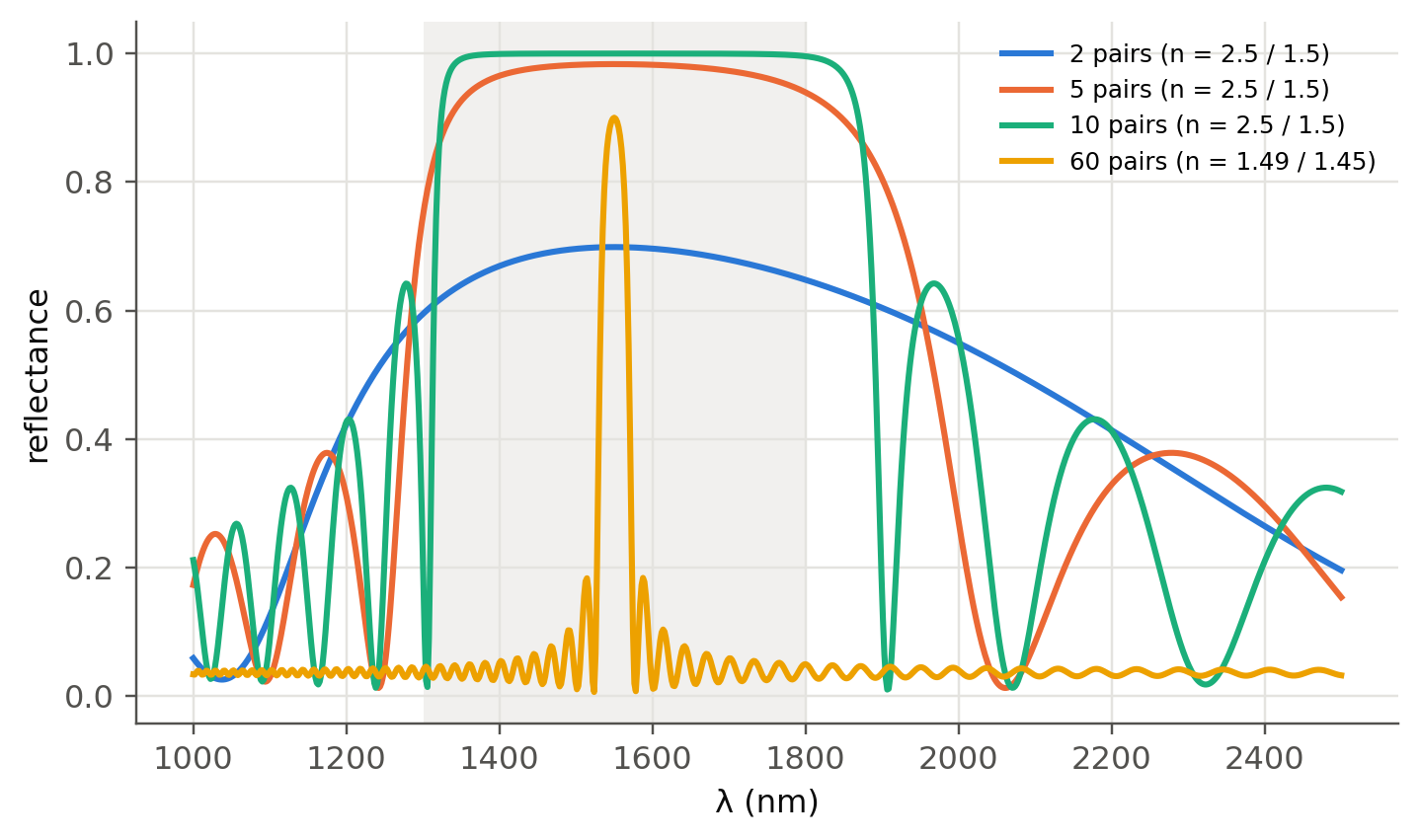
The cladding alternates layers of index $n_1$ and $n_2$. Reflections add in phase when
$n_1d_1+n_2d_2=m\lambda/2$. The usual quarter-wave design is $n_1d_1=n_2d_2=\lambda/4$. Locally, at normal
incidence, the cladding behaves like a planar dielectric mirror. We can therefore compute its reflectance with
the **transfer-matrix method**:
```{python}
#| label: fig-bragg-mirror
#| fig-cap: "Reflectance of a quarter-wave stack (planar approximation of the Bragg-fiber cladding) designed for 1550 nm, for several numbers of layer pairs. Inside the stop band (photonic band gap) the light cannot escape the core."
def stack_R(lam, n_hi, n_lo, N, lam0, n_in=1.0, n_out=1.45):
    d_hi, d_lo = lam0 / (4 * n_hi), lam0 / (4 * n_lo)
    R = []
    for l in lam:
        M = np.eye(2, dtype=complex)
        for n, d in [(n_hi, d_hi), (n_lo, d_lo)] * N:
            ph = 2 * np.pi * n * d / l
            M = M @ np.array([[np.cos(ph), 1j * np.sin(ph) / n], [1j * n * np.sin(ph), np.cos(ph)]])
        B, C = M @ np.array([1, n_out])
        r = (n_in * B - C) / (n_in * B + C)
        R.append(abs(r) ** 2)
    return np.array(R)

lam = np.linspace(1000, 2500, 800) * 1e-9
fig, ax = plt.subplots()
for k, N in enumerate([2, 5, 10]):
    ax.plot(lam * 1e9, stack_R(lam, 2.5, 1.5, N, 1550e-9), color=fl.PALETTE[k], label=f"{N} pairs (n = 2.5 / 1.5)")
ax.plot(lam * 1e9, stack_R(lam, 1.49, 1.45, 60, 1550e-9), color=fl.PALETTE[3], label="60 pairs (n = 1.49 / 1.45)")
dl = 4 / np.pi * np.arcsin((2.5 - 1.5) / (2.5 + 1.5)) * 1550
ax.axvspan(1550 - dl / 2, 1550 + dl / 2, color=fl.GRID, alpha=0.5, lw=0)
ax.set_xlabel("λ (nm)"); ax.set_ylabel("reflectance"); ax.legend(fontsize=8)
plt.show()
print(f"Stop-band width (high contrast): Δλ ≈ (4/π)·asin((n_H−n_L)/(n_H+n_L))·λ0 = {dl:.0f} nm")
```
The core of a Bragg fiber can even be **hollow**. Only a high-contrast cladding gives a wide stop band, which is
why hollow Bragg fibers use polymer/chalcogenide layers.
## Photonic crystal fibers (slides 199–207)
| | solid-core PCF | hollow-core PCF / anti-resonant |
|---|---|---|
| guiding | modified TIR (air holes lower the effective cladding index) | photonic band gap or anti-resonance |
| key property | endlessly single-mode, large NA, engineerable dispersion | ~99.9 % of light in air: tiny nonlinearity and latency, almost no material dispersion |
| applications | supercontinuum, high-power lasers, sensing | low-latency links, high-power delivery, gas spectroscopy |
::: {.callout-note}
## Update since the slides were written
Hollow-core **nested anti-resonant** fibers (NANF/DNANF) have been reported with attenuation **below 0.1 dB/km**
around 1550 nm. That is lower than the Rayleigh limit of silica computed in @sec-attenuation, and the propagation is
~1.5 µs/km faster than in solid glass. They are being deployed in low-latency links (finance, data centres).
:::
## Fiber Bragg gratings (slides 209–213)
A periodic modulation $\Delta n$ of period $\Lambda$ written in the core reflects the **Bragg wavelength**
$$
\lambda_B=2n_\text{eff}\Lambda .
$$
Coupled-mode theory gives, for a uniform grating of length $L$ with $\kappa=\pi\Delta n/\lambda$:
$$
R_\text{max}=\tanh^2(\kappa L),\qquad
\Delta\lambda_0=\frac{\lambda_B^2}{\pi n_\text{eff}L}\sqrt{(\kappa L)^2+\pi^2}\ \ (\text{between first zeros}).
$$
$\kappa L<1$ is a weak grating (narrow, low $R$). $\kappa L>1$ is a strong grating (flat-top, $R\to1$, width set by $\Delta n$).
### Example: FBG at 1550 nm (slide 222)
```{python}
lB, neff, dn, L = 1550e-9, 1.455, 1e-4, 10e-3
Lam = lB / (2 * neff)
kap = np.pi * dn / lB
wl = np.linspace(1549e-9, 1551e-9, 40001)
R = fl.fbg_reflectance(wl, lB, neff, dn, L)
m = R >= R.max() / 2
print(f"Λ = {Lam*1e9:.1f} nm (with n = 1.450 as on the slide: {lB/2/1.450*1e9:.1f} nm)")
print(f"κ = {kap:.1f} m⁻¹, κL = {kap*L:.3f} → strong grating, R_max = tanh²(κL) = {np.tanh(kap*L)**2:.3f}")
print(f"Δλ between first zeros = {fl.fbg_bandwidth(lB, neff, dn, L)*1e9:.3f} nm, FWHM = {(wl[m][-1]-wl[m][0])*1e9:.3f} nm")
```
::: {.callout-warning}
## To double-check on slide 222
The reflectance (93.3 %) matches. The coupled-mode bandwidth formula above gives **≈ 0.20 nm** (0.15 nm FWHM) with these
numbers, whereas the slide quotes 0.428 nm. It is worth verifying which expression or values were used there.
:::
### FBG designer, live
```{ojs}
//| echo: false
viewof fbg = Inputs.form({
  dn: Inputs.range([0.1, 20], {value: 1, step: 0.1, label: "Δn (×10⁻⁴)"}),
  L:  Inputs.range([0.5, 50], {value: 10, step: 0.5, label: "length L (mm)"}),
  lamB: Inputs.range([1500, 1600], {value: 1550, step: 0.5, label: "λ_B (nm)"}),
  eps: Inputs.range([-2000, 2000], {value: 0, step: 50, label: "strain (µε)"}),
  dT: Inputs.range([-100, 200], {value: 0, step: 5, label: "ΔT (K)"})
})
```
```{ojs}
//| echo: false
fbgSpec = {
  const n = 1.455, dn = fbg.dn * 1e-4, L = fbg.L * 1e-3;
  const shift = fbg.lamB * ((1 - 0.22) * fbg.eps * 1e-6 + (0.55e-6 + 6.7e-6) * fbg.dT);   // nm
  const lB = (fbg.lamB + shift) * 1e-9;
  const out = [];
  for (let l = fbg.lamB - 3; l <= fbg.lamB + 3; l += 0.002) {
    const lam = l * 1e-9, k = Math.PI * dn / lam, s = 2 * Math.PI * n * (1/lam - 1/lB);
    let R;
    if (k*k > s*s) { const g = Math.sqrt(k*k - s*s), sh = Math.sinh(g*L), ch = Math.cosh(g*L);
      R = k*k*sh*sh / (k*k*ch*ch - s*s); }
    else { const g = Math.sqrt(s*s - k*k), sn = Math.sin(g*L), cs = Math.cos(g*L);
      R = k*k*sn*sn / (s*s - k*k*cs*cs); }
    out.push({l, R, T: 1 - R});
  }
  return {out, shift, kL: Math.PI * dn / (fbg.lamB*1e-9) * L};
}
Plot.plot({
  width: Math.min(width, 1050), height: 300, x: {label: "λ (nm)"}, y: {label: "reflectance", domain: [0, 1.02], grid: true},
  marks: [Plot.ruleX([fbg.lamB], {stroke: "#b9b8b2", strokeDasharray: "4,3"}),
          Plot.areaY(fbgSpec.out, {x: "l", y: "R", fill: "#2a78d6", fillOpacity: 0.2}),
          Plot.line(fbgSpec.out, {x: "l", y: "R", stroke: "#2a78d6", strokeWidth: 2}),
          Plot.tip(fbgSpec.out, Plot.pointerX({x: "l", y: "R", title: d => `${d.l.toFixed(3)} nm\nR = ${d.R.toFixed(3)}`}))]
})
```
```{ojs}
//| echo: false
html`<div class="result-box">κL = ${fbgSpec.kL.toFixed(2)} (${fbgSpec.kL > 1 ? "strong" : "weak"}) ·
R<sub>max</sub> = ${(100*Math.tanh(fbgSpec.kL)**2).toFixed(1)} % ·
Bragg shift = <b>${(1000*fbgSpec.shift).toFixed(0)} pm</b>
(≈ 1.2 pm/µε and ≈ 11 pm/K at 1550 nm)</div>`
```
### Apodisation (new): getting rid of the side lobes
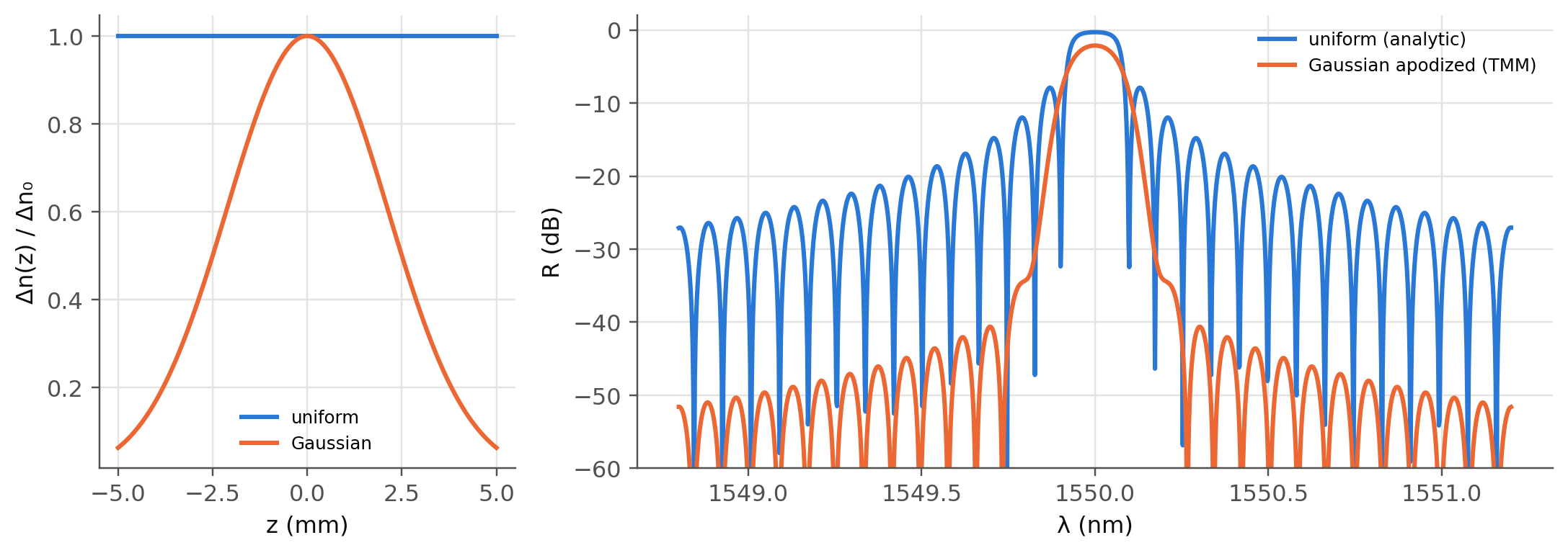
A uniform grating has strong side lobes, which cause crosstalk between DWDM channels. Tapering $\Delta n(z)$ smoothly
suppresses them. We compute non-uniform gratings with the **piecewise-uniform transfer-matrix method** (Erdogan, 1997):
cut the grating into $M$ short uniform sections and multiply their $2\times2$ coupled-mode matrices.
```{python}
#| label: fig-apod
#| fig-cap: "Uniform versus Gaussian-apodized FBG (L = 10 mm, peak Δn = 1e-4), computed with the transfer-matrix method. Apodisation lowers the side lobes by more than 20 dB at the price of a slightly wider main lobe."
def fbg_tmm(wl, lB, neff, dn_z, L):
    M = len(dn_z); dz = L / M
    R = np.empty(len(wl))
    for i, l in enumerate(wl):
        sig = 2 * np.pi * neff * (1 / l - 1 / lB)
        F = np.eye(2, dtype=complex)
        for dn in dn_z:
            k = np.pi * dn / l
            g = np.sqrt(complex(k**2 - sig**2))
            ch, sh = np.cosh(g * dz), (np.sinh(g * dz) / g if abs(g) > 1e-12 else dz)
            Fi = np.array([[ch - 1j * sig * sh, -1j * k * sh], [1j * k * sh, ch + 1j * sig * sh]])
            F = Fi @ F
        R[i] = abs(F[1, 0] / F[0, 0]) ** 2
    return R

wl = np.linspace(1548.8e-9, 1551.2e-9, 1200)
z = np.linspace(-0.5, 0.5, 120)
uni = fl.fbg_reflectance(wl, lB, neff, 1e-4, L)
gau = fbg_tmm(wl, lB, neff, 1e-4 * np.exp(-4 * np.log(2) * (z / 0.5) ** 2), L)
fig, (a1, a2) = plt.subplots(1, 2, figsize=(10, 3.6), gridspec_kw={"width_ratios": [1, 2.2]})
a1.plot(z * 10, np.ones_like(z), label="uniform"); a1.plot(z * 10, np.exp(-4 * np.log(2) * (z / 0.5) ** 2), label="Gaussian")
a1.set_xlabel("z (mm)"); a1.set_ylabel("Δn(z) / Δn₀"); a1.legend(fontsize=8)
a2.plot(wl * 1e9, 10 * np.log10(uni + 1e-9), label="uniform (analytic)")
a2.plot(wl * 1e9, 10 * np.log10(gau + 1e-9), label="Gaussian apodized (TMM)")
a2.set_ylim(-60, 2); a2.set_xlabel("λ (nm)"); a2.set_ylabel("R (dB)"); a2.legend(fontsize=8)
plt.tight_layout(); plt.show()
```
## FBG sensors (slides 214–227)
Strain changes both $\Lambda$ and $n_\text{eff}$ (photo-elastic effect, $p_e\approx0.22$). Temperature changes them through
thermal expansion $\alpha_\Lambda$ and the thermo-optic coefficient $\xi$:
$$
\frac{\Delta\lambda_B}{\lambda_B}=(1-p_e)\,\varepsilon+(\alpha_\Lambda+\xi)\,\Delta T .
$$
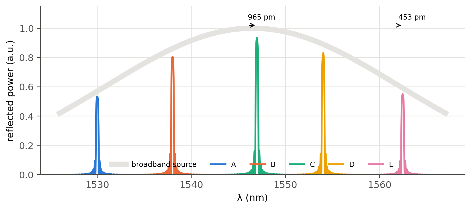
Several gratings at different $\lambda_B$ on one fiber can be read by a single broadband source: this is
**wavelength-division multiplexed sensing** (slides 221, 225).
```{python}
#| label: fig-fbg-array
#| fig-cap: "Five FBG sensors multiplexed in wavelength on one fiber. Sensor C is strained by +800 µε and sensor E heated by +40 K. Each shifts inside its own spectral slot."
centers = np.array([1530, 1538, 1546, 1554, 1562]) * 1e-9
shifts = [(0, 0), (0, 0), (800e-6, 0), (0, 0), (0, 40)]
wl = np.linspace(1526e-9, 1567e-9, 6000)
fig, ax = plt.subplots(figsize=(8.5, 3.4))
ax.plot(wl * 1e9, np.exp(-((wl - 1546.5e-9) / 22e-9) ** 2), color=fl.GRID, lw=6, label="broadband source")
for k, (c, (eps, dT)) in enumerate(zip(centers, shifts)):
    lb = c * (1 + 0.78 * eps + 7.25e-6 * dT)
    Rk = fl.fbg_reflectance(wl, lb, 1.455, 2e-4, 5e-3)
    ax.plot(wl * 1e9, Rk * np.exp(-((lb - 1546.5e-9) / 22e-9) ** 2), color=fl.PALETTE[k], label="ABCDE"[k])
    if lb != c:
        ax.annotate("", xy=(lb * 1e9, 1.02), xytext=(c * 1e9, 1.02), arrowprops=dict(arrowstyle="->", color=fl.INK))
        ax.text(c * 1e9, 1.06, f"{(lb-c)*1e12:.0f} pm", fontsize=8)
ax.set_xlabel("λ (nm)"); ax.set_ylabel("reflected power (a.u.)"); ax.legend(ncol=6, fontsize=8, loc="lower center")
ax.set_ylim(0, 1.15); plt.show()
```
## Try it yourself
1. Use `fbg_tmm` with a **linear chirp** of $\Lambda(z)$. Show that the reflected group delay varies linearly with
$\lambda$. A chirped FBG is a compact **dispersion compensator** (@sec-dispersion).
2. Add a $\pi$ phase shift in the middle of the grating. What appears at $\lambda_B$?
3. How can you separate strain from temperature with FBGs? (Hint: two gratings, one strain-free, or two gratings
with different sensitivities.)