# Step-index optical fibers {#sec-fibers}
[](https://colab.research.google.com/github/{{< var github_user >}}/{{< var repo >}}/blob/main/{{< var subdir >}}/notebooks/fibers.ipynb){.colab-link} Run this chapter's code in Google Colab (no installation).
```{python}
#| include: false
import numpy as np
import matplotlib.pyplot as plt
import fiberlib as fl
fl.use_style()
c0 = fl.c0
```
*Slides 40–64.* A cylindrical core of radius $a$ and index $n_1$, inside a cladding of index $n_2$.
Two kinds of rays appear (slide 42). **Meridional** rays cross the axis. **Skew** rays spiral
around it. In the wave picture the two families give the **LP$_{lm}$** modes.
## Weakly guiding fibers and LP modes (slides 43–47)
When $\Delta\ll1$ (typically 0.3 % to 2 %), the guided modes are almost transverse and linearly polarised:
$$
E_{LP}=E_{lm}(r,\phi)\,e^{j(\omega t-\beta_{lm}z)},\qquad
E_{lm}(r,\phi)=f(r)\cos(l\phi)\ \text{or}\ f(r)\sin(l\phi).
$$
Inside the core $f(r)\propto J_l(ur/a)$ and in the cladding $f(r)\propto K_l(wr/a)$, with
$u^2+w^2=V^2$. Continuity of $f$ and $f'$ at $r=a$ gives the **eigenvalue equation**
$$
\frac{u\,J_{l-1}(u)}{J_l(u)}=-\frac{w\,K_{l-1}(w)}{K_l(w)} .
$$ {#eq-lp}
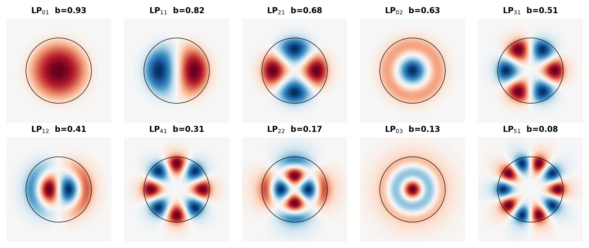
The mode index $l$ sets the azimuthal order ($2l$ maxima around a circle). The index $m$ counts the
radial maxima. The function `fl.LP_b(V, l, m)` solves @eq-lp, and you can read it in
[`fiberlib.py`](fiberlib.py): it is a sign-change scan followed by Brent's method.
```{python}
for l, m, b in fl.LP_all(5.0):
    print(f"LP{l}{m}:  b = {b:.4f}")
print("Guided modes incl. polarisation and orientation:", fl.LP_count(5.0), " (V²/2 =", 5**2/2, ")")
```
### The $b$–$V$ chart (slide 49)
```{python}
#| label: fig-bV
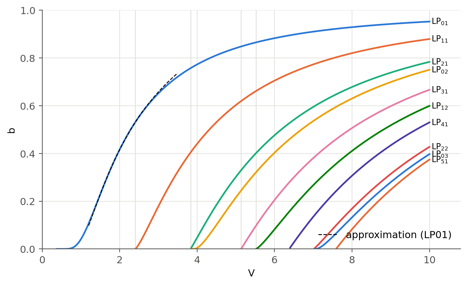
#| fig-cap: "Normalized propagation constant b(V) of the first LP modes (exact solution of the weak-guidance eigenvalue equation). The dashed line is the LP01 approximation b ≈ (1.1428 − 0.996/V)², good for 1.5 < V < 2.5."
Vg = np.linspace(0.3, 10, 400)
modes = [(0,1),(1,1),(2,1),(0,2),(3,1),(1,2),(4,1),(2,2),(0,3),(5,1)]
curves = {}
fig, ax = plt.subplots(figsize=(8, 4.6))
for k, (l, m) in enumerate(modes):
    b = np.array([fl.LP_b(V, l, m) for V in Vg])
    curves[f"LP{l}{m}"] = b
    ok = np.isfinite(b)
    ax.plot(Vg[ok], b[ok], color=fl.PALETTE[k % 8], lw=1.8)
    i = np.where(ok)[0][-1]
    ax.text(Vg[i] + 0.05, b[i], f"LP$_{{{l}{m}}}$", fontsize=8.5, va="center")
Va = np.linspace(1.2, 3.5, 100)
ax.plot(Va, fl.b_approx(Va), "--", color=fl.INK, lw=1, label="approximation (LP01)")
for vc in [2.405, 3.832, 5.136, 5.520]:
    ax.axvline(vc, color=fl.GRID, lw=1, zorder=0)
ax.set_xlabel("V"); ax.set_ylabel("b"); ax.set_ylim(0, 1); ax.set_xlim(0, 10.8)
ax.legend(loc="lower right")
plt.show()
```
The cut-offs are zeros of Bessel functions. LP$_{0m}$ is cut off at the zeros of $J_1$
(0, 3.832, 7.016 …). LP$_{lm}$ with $l\ge1$ is cut off at the zeros of $J_{l-1}$, which gives 2.405 for LP$_{11}$.
Below you can sweep $V$ and see which modes are guided, together with their $b$ and effective index.
```{python}
#| echo: false
ojs_define(bV={"V": Vg.tolist(), **{k: np.nan_to_num(v, nan=-1).tolist() for k, v in curves.items()}})
```
```{ojs}
//| echo: false
viewof Vfib = Inputs.range([0.5, 10], {value: 2.2, step: 0.01, label: "V-number"})
```
```{ojs}
//| echo: false
bVlong = Object.keys(bV).filter(k => k !== "V").flatMap(k => bV.V.map((v, i) => ({V: v, b: bV[k][i], mode: k}))).filter(d => d.b >= 0)
bAtV = Object.keys(bV).filter(k => k !== "V").map(k => {
  const i = d3.bisectLeft(bV.V, Vfib); const i0 = Math.max(1, Math.min(i, bV.V.length - 1));
  const t = (Vfib - bV.V[i0-1]) / (bV.V[i0] - bV.V[i0-1]);
  const b0 = bV[k][i0-1], b1 = bV[k][i0];
  return {mode: k, b: (b0 < 0 || b1 < 0) ? -1 : b0 + t * (b1 - b0)};
}).filter(d => d.b > 0)
Plot.plot({
  width: Math.min(width, 1050), height: 360, x: {label: "V", domain: [0, 10]}, y: {label: "b", domain: [0, 1]},
  marks: [
    Plot.line(bVlong, {x: "V", y: "b", z: "mode", stroke: "#b9b8b2", strokeWidth: 1.5}),
    Plot.ruleX([Vfib], {stroke: "#2a78d6", strokeWidth: 2}),
    Plot.dot(bAtV, {x: () => Vfib, y: "b", r: 5, fill: "#2a78d6", stroke: "white", strokeWidth: 2, tip: true,
                    title: d => `${d.mode}  b = ${d.b.toFixed(4)}`}),
    Plot.text(bAtV, {x: () => Vfib, y: "b", text: "mode", dx: 10, textAnchor: "start", fontWeight: "bold"})
  ]
})
```
```{ojs}
//| echo: false
html`<div class="result-box">V = ${Vfib.toFixed(2)}: <b>${bAtV.length} LP mode(s)</b> (${bAtV.map(d => d.mode).join(", ")})
 · total with degeneracies ≈ ${bAtV.reduce((s, d) => s + (d.mode[2] === "0" ? 2 : 4), 0)}
 · V²/2 = ${(Vfib*Vfib/2).toFixed(1)}
 ${Vfib < 2.405 ? "· <b>single-mode</b>" : ""}</div>`
```
### What the modes look like (slides 44–47)
```{python}
#| label: fig-lp-maps
#| fig-cap: "Transverse field E(x,y) of the LP modes guided at V = 8 (cos lφ orientation). Red and blue are opposite signs. The circle marks the core."
V = 8.0
allm = fl.LP_all(V)
x = np.linspace(-1.6, 1.6, 241)
X, Y = np.meshgrid(x, x)
R, PHI = np.hypot(X, Y), np.arctan2(Y, X)
n = len(allm); cols = 5; rows = int(np.ceil(n / cols))
fig, axs = plt.subplots(rows, cols, figsize=(1.9 * cols, 2.0 * rows))
for ax in axs.flat: ax.axis("off")
for ax, (l, m, b) in zip(axs.flat, allm):
    E = fl.LP_field(R, V, b, l) * np.cos(l * PHI)
    E /= np.abs(E).max()
    ax.imshow(E, cmap="RdBu_r", vmin=-1, vmax=1, extent=[-1.6, 1.6, -1.6, 1.6])
    ax.add_patch(plt.Circle((0, 0), 1, fill=False, color="k", lw=0.6))
    ax.set_title(f"LP$_{{{l}{m}}}$  b={b:.2f}", fontsize=9)
plt.tight_layout(); plt.show()
```
```{python}
#| label: fig-lp-irr
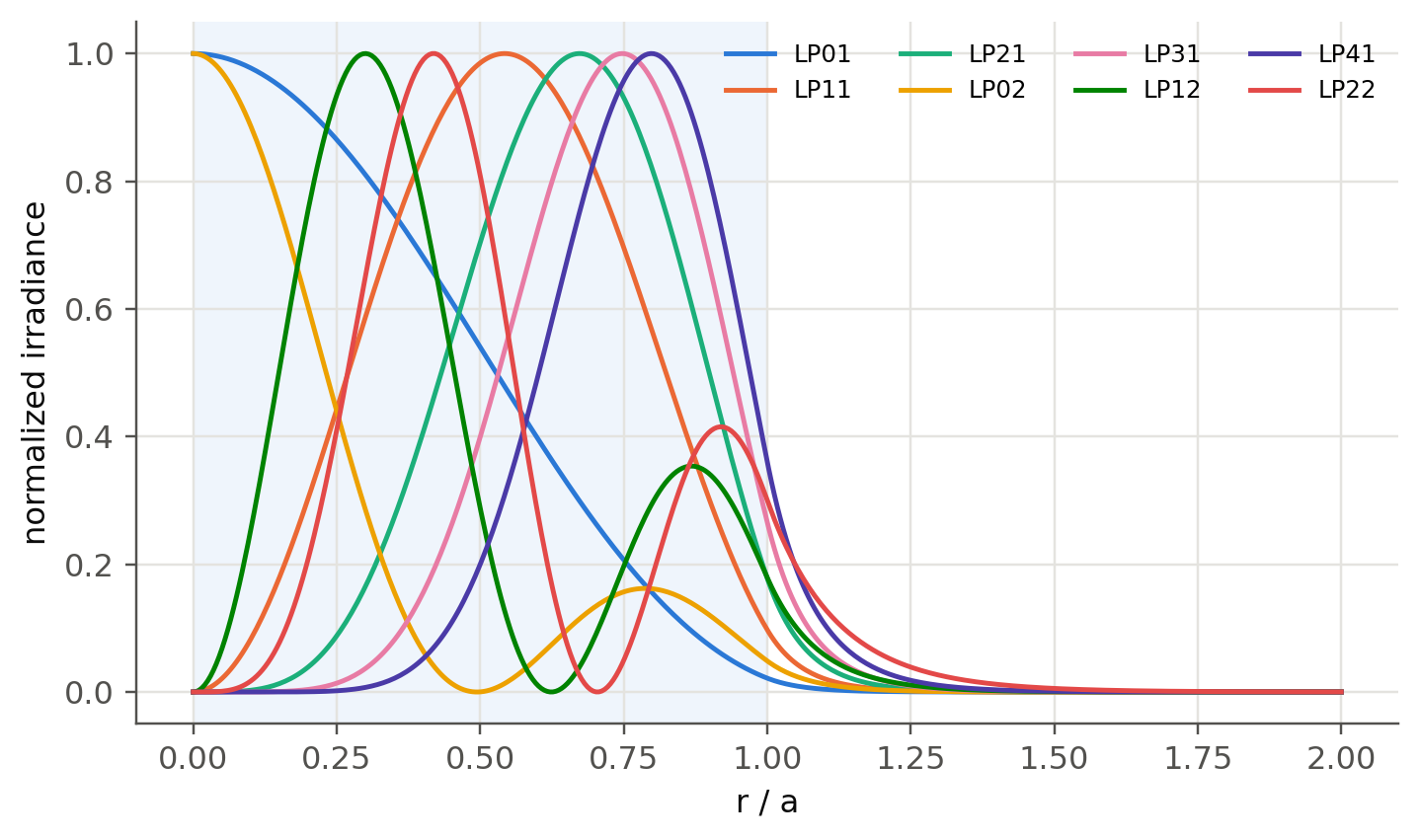
#| fig-cap: "Radial irradiance |f(r)|² of the guided LP modes at V = 8, normalized to the core boundary value. Low-b modes reach far into the cladding."
r = np.linspace(0, 2, 400)
fig, ax = plt.subplots()
ax.axvspan(0, 1, color=fl.PALETTE[0], alpha=0.07, lw=0)
for k, (l, m, b) in enumerate(allm[:8]):
    I = fl.LP_field(r, V, b, l) ** 2
    ax.plot(r, I / I.max(), color=fl.PALETTE[k], lw=1.6, label=f"LP{l}{m}")
ax.set_xlabel("r / a"); ax.set_ylabel("normalized irradiance"); ax.legend(ncol=4, fontsize=8)
plt.show()
```
## Fiber parameters (slides 48, 61–62)
| quantity | formula |
|---|---|
| normalized index difference | $\Delta = \dfrac{n_1^2-n_2^2}{2n_1^2}\approx\dfrac{n_1-n_2}{n_1}$ |
| numerical aperture | $\mathrm{NA}=\sqrt{n_1^2-n_2^2}\approx n_1\sqrt{2\Delta}$ |
| acceptance angle | $\sin\alpha_\text{max} = \mathrm{NA}/n_0$ |
| $V$-number | $V=\dfrac{2\pi a}{\lambda}\,\mathrm{NA}$ |
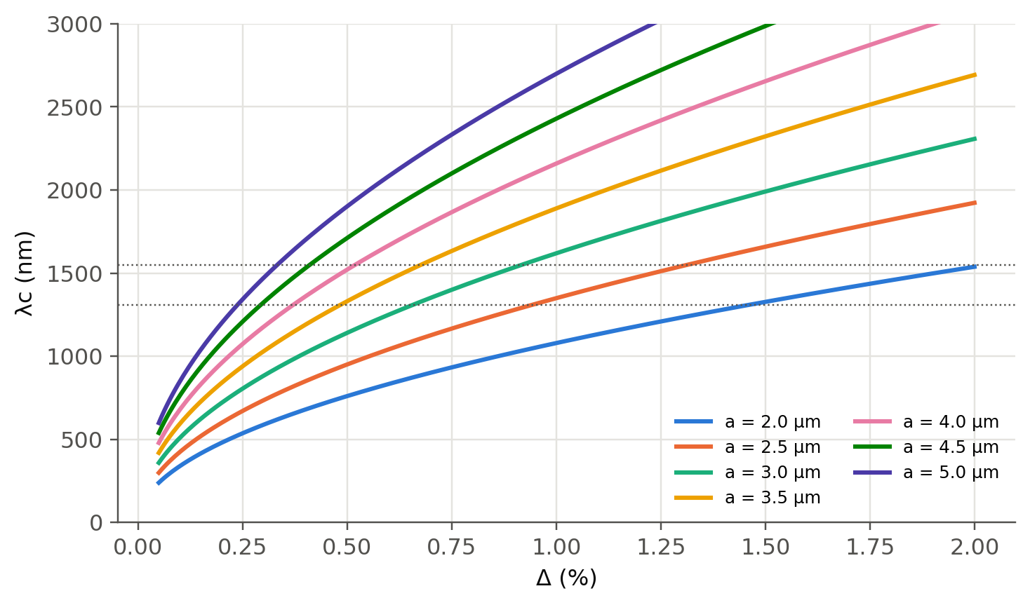
| single mode | $V<2.405$, i.e. $\lambda>\lambda_c=\dfrac{2\pi a\,\mathrm{NA}}{2.405}$ |
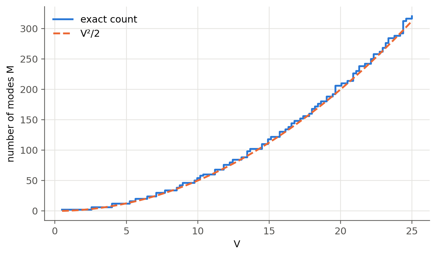
| number of modes ($V\gg1$) | $M\approx V^2/2$ |
```{python}
#| label: fig-nmodes
#| fig-cap: "Exact number of guided modes (both polarisations, both orientations) compared with V²/2."
Vs = np.linspace(0.5, 25, 120)
Mex = [fl.LP_count(v) for v in Vs]
fig, ax = plt.subplots()
ax.step(Vs, Mex, where="post", label="exact count")
ax.plot(Vs, Vs**2 / 2, "--", color=fl.PALETTE[1], label="V²/2")
ax.set_xlabel("V"); ax.set_ylabel("number of modes M"); ax.legend()
plt.show()
```
### Single-mode cut-off vs. index contrast (from `ofiber_test.ipynb`)
```{python}
#| label: fig-cutoff
#| fig-cap: "Cut-off wavelength of a step-index fiber versus Δ for several core radii (n2 = 1.45)."
n_clad = 1.45
D = np.linspace(0.0005, 0.02, 300)
n_core = n_clad / (1 - D)
fig, ax = plt.subplots()
for k, a in enumerate(np.array([2, 2.5, 3, 3.5, 4, 4.5, 5]) * 1e-6):
    lc = 2 * np.pi * a * fl.NA(n_core, n_clad) / 2.405
    ax.plot(D * 100, lc * 1e9, color=fl.PALETTE[k], label=f"a = {a*1e6:.1f} µm")
for lam in (1310, 1550):
    ax.axhline(lam, color=fl.INK2, lw=0.8, ls=":")
ax.set_xlabel("Δ (%)"); ax.set_ylabel("λc (nm)"); ax.set_ylim(0, 3000); ax.legend(ncol=2, fontsize=8)
plt.show()
```
## Live fiber designer
Type the fiber parameters and all the quantities of slides 48–64 update. You can also use this panel to
check every worked example below.
```{ojs}
//| echo: false
viewof fd = Inputs.form({
  n1: Inputs.number([1.3, 1.7], {value: 1.4532, step: 0.0001, label: "core index n₁"}),
  n2: Inputs.number([1.3, 1.7], {value: 1.4485, step: 0.0001, label: "cladding index n₂"}),
  d:  Inputs.number([1, 1000], {value: 8.2, step: 0.1, label: "core diameter 2a (µm)"}),
  lam: Inputs.number([0.3, 2.5], {value: 1.31, step: 0.01, label: "wavelength λ (µm)"})
})
```
```{ojs}
//| echo: false
fiberOut = {
  const {n1, n2, d, lam} = fd, a = d / 2;
  if (!(n1 > n2)) return null;
  const NAv = Math.sqrt(n1*n1 - n2*n2), Dl = (n1*n1 - n2*n2) / (2*n1*n1);
  const V = 2*Math.PI*a/lam*NAv, lc = 2*Math.PI*a*NAv/2.405;
  const mfd = 2*a*(0.65 + 1.619*Math.pow(V, -1.5) + 2.879*Math.pow(V, -6));
  return {NAv, Dl, V, lc, mfd, amax: Math.asin(Math.min(NAv, 1)) * 180/Math.PI, M: V*V/2,
          dtau: (n1 - n2) / 299792458 * 1e3 * 1e9};
}
fiberOut === null ? html`<div class="result-box">n₁ must be larger than n₂.</div>` :
html`<div class="result-box">
Δ = ${(100*fiberOut.Dl).toFixed(3)} % · NA = ${fiberOut.NAv.toFixed(4)} ·
α<sub>max</sub> = ${fiberOut.amax.toFixed(2)}° (total 2α<sub>max</sub> = ${(2*fiberOut.amax).toFixed(1)}°)<br>
V = <b>${fiberOut.V.toFixed(3)}</b> → ${fiberOut.V < 2.405 ? "<b>single-mode</b>" : `<b>multimode</b>, M ≈ V²/2 ≈ ${Math.round(fiberOut.M)}`}<br>
cut-off wavelength λ<sub>c</sub> = ${(1000*fiberOut.lc).toFixed(0)} nm<br>
${fiberOut.V > 0.8 && fiberOut.V < 2.6 ? `MFD (Marcuse) = ${fiberOut.mfd.toFixed(2)} µm · ` : ""}
step-index intermodal spread ≈ ${fiberOut.dtau.toFixed(1)} ns/km
</div>`
```
## Worked examples (slides 51–64), recomputed
```{python}
def report(title, **kv):
    print(f"── {title}")
    for k, v in kv.items(): print(f"   {k:<28s} {v}")

# Slide 57 — multimode fiber
V = fl.V_number(50e-6, 0.85e-6, 1.468, 1.447)
report("Slide 57: MMF, 2a = 100 µm, λ = 850 nm", V=f"{V:.2f}", **{"M ≈ V²/2": f"{V**2/2:.0f}",
       "exact count": fl.LP_count(V)})

# Slide 58 — maximum radius for SMF at 1.3 µm
a_max = 2.405 * 1.3e-6 / (2 * np.pi * fl.NA(1.468, 1.447))
report("Slide 58: SMF core radius at 1.3 µm", **{"a ≤": f"{a_max*1e6:.2f} µm"})

# Slides 59-60 — cut-off and MFD
a, n1, n2 = 4.1e-6, 1.4532, 1.4485
lc = 2 * np.pi * a * fl.NA(n1, n2) / 2.405
V = fl.V_number(a, 1.31e-6, n1, n2)
report("Slides 59–60: 2a = 8.2 µm at 1.31 µm", **{
    "λc": f"{lc*1e6:.3f} µm", "V": f"{V:.3f}",
    "MFD Marcuse": f"{fl.mfd_marcuse(a, V)*1e6:.2f} µm",
    "MFD 2a(2.6/V)": f"{2*a*2.6/V*1e6:.2f} µm",
    "MFD exact Gaussian fit (new)": f"{fl.mfd_exact_gaussian(a, V)*1e6:.2f} µm",
    "MFD Petermann II (ITU, new)": f"{fl.mfd_petermann2(a, V)*1e6:.2f} µm"})

# Slide 63 — NA and acceptance
n1, n2 = 1.480, 1.460
NAv = fl.NA(n1, n2); V = fl.V_number(50e-6, 0.85e-6, n1, n2)
report("Slide 63: MMF NA", NA=f"{NAv:.4f}", **{"α_max": f"{np.degrees(np.arcsin(NAv)):.1f}°",
       "2α_max": f"{2*np.degrees(np.arcsin(NAv)):.1f}°", "V": f"{V:.2f}", "M": f"{V**2/2:.0f}",
       "Δ": f"{(n1-n2)/n1*100:.2f} %"})

# Slide 64 — SMF with Δ = 0.3 %
n1, Dl = 1.460, 0.003
NAv = n1 * np.sqrt(2 * Dl)
report("Slide 64: SMF, 2a = 8 µm, Δ = 0.3 %", NA=f"{NAv:.3f}",
       **{"2α_max": f"{2*np.degrees(np.arcsin(NAv)):.1f}°", "λc": f"{2*np.pi*4e-6*NAv/2.405*1e6:.2f} µm"})
```
### Group velocity and group delay (slides 51–52)
> SMF with $n_1=1.4480$, $n_2=1.4400$, $a=3$ µm at $\lambda=1.5$ µm. What are $v_g$ and the group delay
> over 1 km? Neglect material dispersion.
The slides use $\beta \approx n_2k[1+b\Delta]$ with the approximate $b(V)$, and a 0.1 % finite difference.
We do the same and also use the **exact** $b(V)$ and an exact derivative.
```{python}
n1, n2, a = 1.4480, 1.4400, 3e-6
Dl = (n1 - n2) / n1
def beta(wl, exact):
    V = fl.V_number(a, wl, n1, n2)
    b = fl.LP_b(V, 0, 1) if exact else fl.b_approx(V)
    return n2 * 2 * np.pi / wl * (1 + b * Dl)
for exact, h in [(False, 1.5e-9), (True, 1e-12)]:
    w1, w2 = 1.5e-6, 1.5e-6 + h
    om = lambda wl: 2 * np.pi * c0 / wl
    vg = (om(w1) - om(w2)) / (beta(w1, exact) - beta(w2, exact))
    print(f"{'exact b(V), dλ→0' if exact else 'approx. b(V), dλ = 0.1%':<26s}: "
          f"b = {fl.LP_b(fl.V_number(a,w1,n1,n2),0,1) if exact else fl.b_approx(fl.V_number(a,w1,n1,n2)):.5f}, "
          f"v_g = {vg:.5e} m/s, τ_g(1 km) = {1e3/vg*1e6:.4f} µs")
```
## Mode field diameter (slides 53–56)
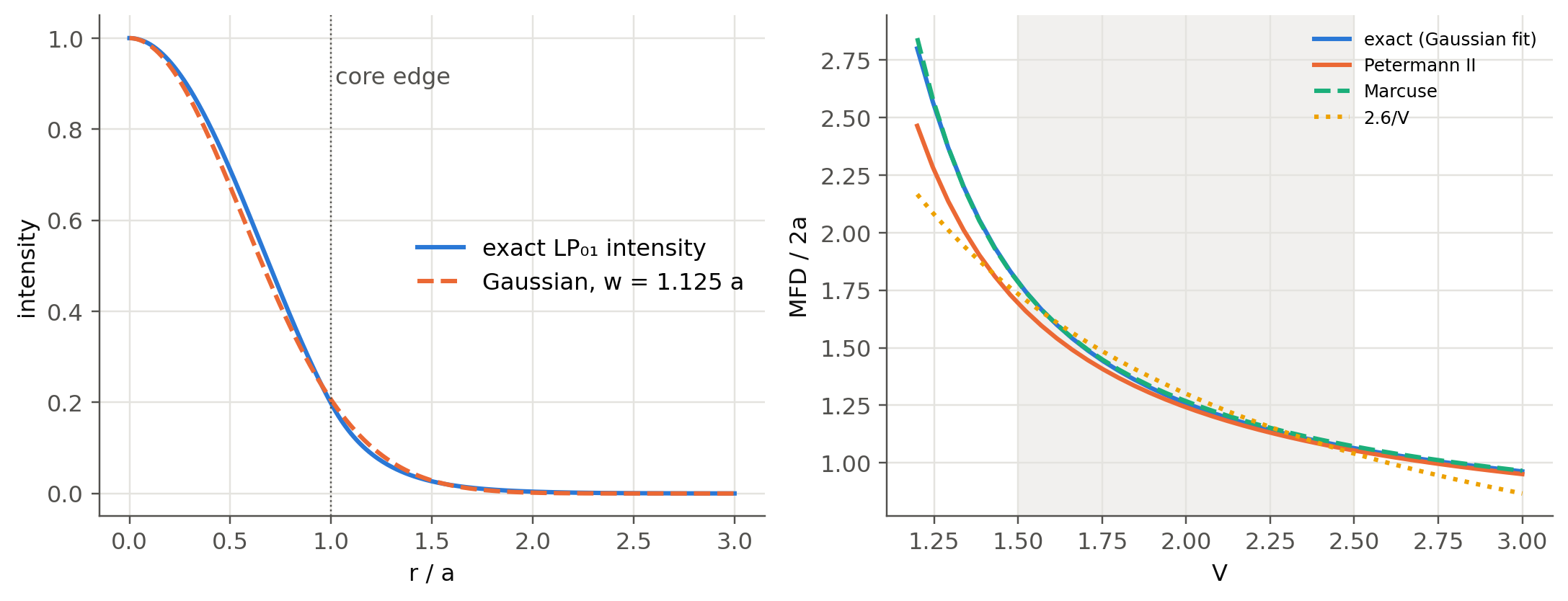
The LP$_{01}$ field is very close to a Gaussian $E\propto\exp(-r^2/w^2)$. The MFD is $2w$. Because the
intensity is Gaussian, the fraction of power inside $r<w$ is $1-e^{-2}\approx 86\,\%$, just like a
Gaussian beam (Chapter 1).
```{python}
#| label: fig-mfd
#| fig-cap: "Left: exact LP01 field at V = 2.30 and its best Gaussian fit. Right: MFD/2a versus V from three definitions. Marcuse's formula is excellent for 1.5 < V < 2.5. The simple 2.6/V rule is not."
fig, (ax1, ax2) = plt.subplots(1, 2, figsize=(10, 3.9))
V = 2.30; b = fl.LP_b(V, 0, 1)
r = np.linspace(0, 3, 400)
E = fl.LP_field(r, V, b, 0); E /= E[0]
w = fl.mfd_exact_gaussian(1, V) / 2
ax1.plot(r, E**2, label="exact LP₀₁ intensity")
ax1.plot(r, np.exp(-2 * (r / w) ** 2), "--", label=f"Gaussian, w = {w:.3f} a")
ax1.axvline(1, color=fl.INK2, lw=0.8, ls=":"); ax1.text(1.02, 0.9, "core edge", color=fl.INK2)
ax1.set_xlabel("r / a"); ax1.set_ylabel("intensity"); ax1.legend()
Vs = np.linspace(1.2, 3.0, 40)
ax2.plot(Vs, [fl.mfd_exact_gaussian(1, v) / 2 for v in Vs], label="exact (Gaussian fit)")
ax2.plot(Vs, [fl.mfd_petermann2(1, v) / 2 for v in Vs], label="Petermann II")
ax2.plot(Vs, fl.mfd_marcuse(1, Vs) / 2, "--", label="Marcuse")
ax2.plot(Vs, 2.6 / Vs, ":", label="2.6/V")
ax2.axvspan(1.5, 2.5, color=fl.GRID, alpha=0.5, lw=0)
ax2.set_xlabel("V"); ax2.set_ylabel("MFD / 2a"); ax2.legend(fontsize=8)
plt.tight_layout(); plt.show()
```
### $V$ across the telecom band (from `ofiber_test.ipynb`)
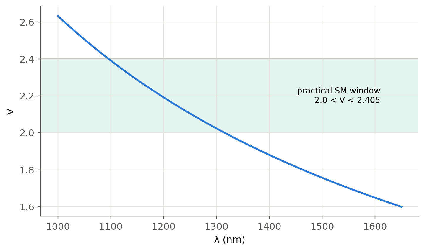
The indices themselves depend on $\lambda$ (Sellmeier, see @sec-dispersion). Here is $V(\lambda)$ for a 9 µm
core of SiO$_2$ doped with 2 % GeO$_2$ inside a pure-silica cladding:
```{python}
#| label: fig-V-lambda
#| fig-cap: "V-number versus wavelength for 2a = 9 µm, core SiO2 + 2 mol% GeO2, cladding pure SiO2."
lam = np.linspace(1000, 1650, 200) * 1e-9
V = fl.V_number(4.5e-6, lam, fl.n_doped(lam, 0.02), fl.n_silica(lam))
fig, ax = plt.subplots()
ax.plot(lam * 1e9, V)
ax.axhspan(2.0, 2.405, color=fl.PALETTE[2], alpha=0.12, lw=0)
ax.axhline(2.405, color=fl.INK2, lw=0.8)
ax.text(1610, 2.2, "practical SM window\n2.0 < V < 2.405", ha="right", va="center", fontsize=9)
ax.set_xlabel("λ (nm)"); ax.set_ylabel("V")
plt.show()
```
## Try it yourself
1. Modify the 2-D map cell to plot **intensity** of LP$_{11}$ as the sum of its cos and sin variants
with random phases. This is what a speckled multimode output looks like.
2. Check the claim of slide 55: for which $V$ range is Marcuse within 1 % of the exact Gaussian fit?
3. **Exact vector modes (advanced).** LP$_{11}$ is really HE$_{21}$, TE$_{01}$ and TM$_{01}$, which have slightly
different $\beta$. Look up the full eigenvalue equation (Snyder & Love) and plot the splitting versus $\Delta$.
This is the beginning of mode-division multiplexing (MDM) with few-mode fibers.
4. Use the **fiber designer** to design a fiber that is single-mode at 850 nm (VCSEL links), with an MFD
larger than 5 µm.