# Graded-index fibers {#sec-grin}
[](https://colab.research.google.com/github/{{< var github_user >}}/{{< var repo >}}/blob/main/{{< var subdir >}}/notebooks/grin.ipynb){.colab-link} Run this chapter's code in Google Colab (no installation).
```{python}
#| include: false
import numpy as np
import matplotlib.pyplot as plt
from scipy.integrate import solve_ivp
import fiberlib as fl
fl.use_style()
c0 = fl.c0
```
*Slides 122–134.* In a step-index MMF, steep rays travel longer paths and arrive late. If the index
**decreases away from the axis**, those steep rays spend time in faster, low-index glass and can catch up
with the axial ray.
$$
n(r)=n_1\left[1-2\Delta\left(\frac{r}{a}\right)^{\gamma}\right]^{1/2}\ (r<a),\qquad n=n_2\ (r\ge a).
$$
## Ray tracing in a graded core
For a meridional ray, the quantity $\tilde\beta=n(r)\cos\theta(r)$ is conserved (Snell's law for a continuous
stratified medium, slide 123). The trajectory obeys
$$
\frac{d^2x}{dz^2}=\frac{1}{2\tilde\beta^2}\frac{\partial n^2}{\partial x},\qquad
\frac{dt}{dz}=\frac{n^2(x)}{c\,\tilde\beta}.
$$
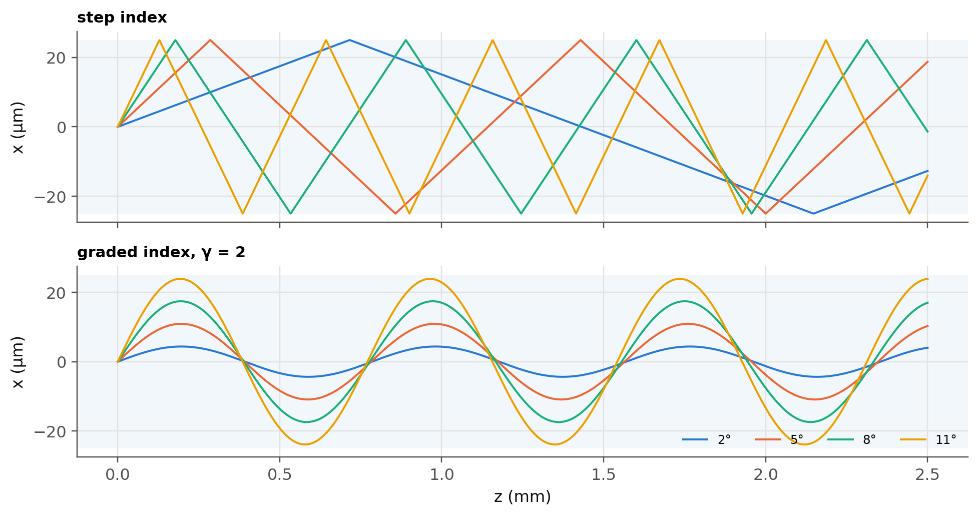
We integrate these equations for rays launched on axis at increasing angles, in a step-index core and in a
parabolic ($\gamma=2$) core with the same $n_1$ and $\Delta$.
```{python}
#| label: fig-rays
#| fig-cap: "Meridional rays launched from the axis at 2°, 5°, 8° and 11° (inside the core) in a step-index fiber (top) and a parabolic GRIN fiber (bottom). The GRIN rays bend smoothly and periodically refocus on the axis."
n1, Dl, a = 1.475, 0.02, 25e-6
n2 = n1 * np.sqrt(1 - 2 * Dl)
def n_prof(x, gamma):
    r = np.minimum(np.abs(x) / a, 1.0)
    return n1 * np.sqrt(1 - 2 * Dl * r**gamma)

def trace_grin(theta0, gamma, zmax):
    bt = n1 * np.cos(theta0)
    def rhs(z, y):
        x, xp, t = y
        h = 1e-9
        dn2 = (n_prof(x + h, gamma)**2 - n_prof(x - h, gamma)**2) / (2 * h)
        return [xp, dn2 / (2 * bt**2), n_prof(x, gamma)**2 / (c0 * bt)]
    s = solve_ivp(rhs, (0, zmax), [0, np.tan(theta0), 0], max_step=zmax / 4000, rtol=1e-10, atol=1e-14)
    return s.t, s.y[0], s.y[2][-1]

def trace_step(theta0, zmax):
    z = np.linspace(0, zmax, 4000)
    period = 4 * a / np.tan(theta0)
    ph = (z / period) % 1
    x = a * np.where(ph < .25, 4 * ph, np.where(ph < .75, 2 - 4 * ph, 4 * ph - 4))
    return z, x

zmax = 2.5e-3
angles = np.radians([2, 5, 8, 11])
fig, axs = plt.subplots(2, 1, figsize=(9, 4.8), sharex=True)
for k, th0 in enumerate(angles):
    z, x = trace_step(th0, zmax); axs[0].plot(z * 1e3, x * 1e6, color=fl.PALETTE[k], lw=1.3)
    z, x, _ = trace_grin(th0, 2, zmax); axs[1].plot(z * 1e3, x * 1e6, color=fl.PALETTE[k], lw=1.3,
                                                    label=f"{np.degrees(th0):.0f}°")
for ax, ttl in zip(axs, ["step index", "graded index, γ = 2"]):
    ax.axhspan(-25, 25, color=fl.PALETTE[0], alpha=0.06, lw=0)
    ax.set_ylabel("x (µm)"); ax.set_title(ttl, loc="left", fontsize=10)
axs[1].set_xlabel("z (mm)"); axs[1].legend(ncol=4, loc="lower right", fontsize=8)
plt.tight_layout(); plt.show()
```
### Who arrives first?
Integrating the ray over a non-integer number of periods biases its average speed. So, for the transit time,
we average exactly over one oscillation, between the axis and the turning point $x_t$ where $n(x_t)=\tilde\beta$:
$$
\frac{\tau}{L}=\frac1c\,\frac{\int_0^{x_t} n^2\,(n^2-\tilde\beta^2)^{-1/2}dx}{\int_0^{x_t}\tilde\beta\,(n^2-\tilde\beta^2)^{-1/2}dx}.
$$
```{python}
#| label: fig-delay
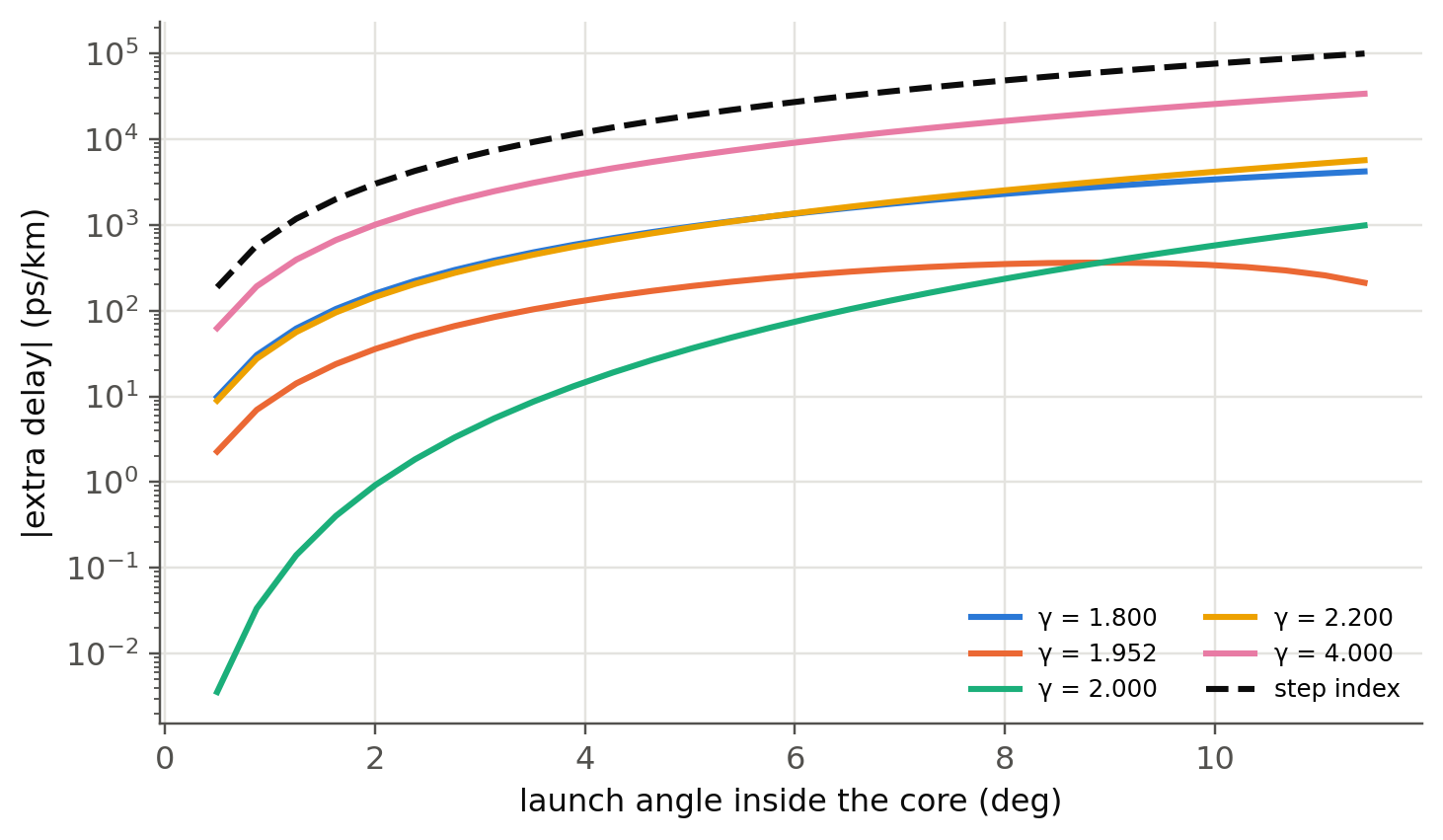
#| fig-cap: "Extra delay per km relative to the axial ray, versus launch angle, for several profile exponents γ (Δ = 2 %). Step index grows like θ². For meridional rays the parabola (γ = 2) is best, with a residual ∝ θ⁴. The wave-theory optimum γ ≈ 2 − 12Δ/5 = 1.952 instead balances all modes, skew rays included. Note the logarithmic scale."
from scipy.integrate import quad
def delay_ps_km(theta0, gamma):
    """Extra delay (ps/km) of a meridional ray vs the axial ray, exact period average.
    With y = x/x_t: n^2 - bt^2 = (n1^2 - bt^2)(1 - y^gamma); substitute y = 1 - s^2."""
    bt = n1 * np.cos(theta0)
    A2 = n1**2 - bt**2
    wdy = lambda s: 2 * s / np.sqrt(-np.expm1(gamma * np.log1p(-s * s))) if s > 0 else 2 / np.sqrt(gamma)
    y = lambda s: 1 - s * s
    num = quad(lambda s: (n1**2 - A2 * y(s)**gamma - n1 * bt) * wdy(s), 0, 1, epsrel=1e-12)[0]
    den = quad(lambda s: bt * wdy(s), 0, 1, epsrel=1e-12)[0]
    return num / den / c0 * 1e3 * 1e12

thetas = np.radians(np.linspace(0.5, np.degrees(np.arccos(n2 / n1)) * 0.99, 30))
fig, ax = plt.subplots()
for k, g in enumerate([1.8, 2 - 12 * Dl / 5, 2.0, 2.2, 4.0]):
    ax.plot(np.degrees(thetas), [abs(delay_ps_km(th, g)) for th in thetas], color=fl.PALETTE[k], label=f"γ = {g:.3f}")
ax.plot(np.degrees(thetas), n1 / c0 * (1 / np.cos(thetas) - 1) * 1e15, "--", color=fl.INK, label="step index")
ax.set_yscale("log")
ax.set_xlabel("launch angle inside the core (deg)"); ax.set_ylabel("|extra delay| (ps/km)")
ax.legend(ncol=2, fontsize=8); plt.show()
```
The ray picture already shows the ~1000× improvement and the sharp optimum. Meridional rays alone, however, do not
see the skew rays, which is why their "best" profile is γ = 2 and not 2 − 12Δ/5. The exact numbers below come from
wave theory, which counts every mode.
## Optimum profile (slides 124–126)
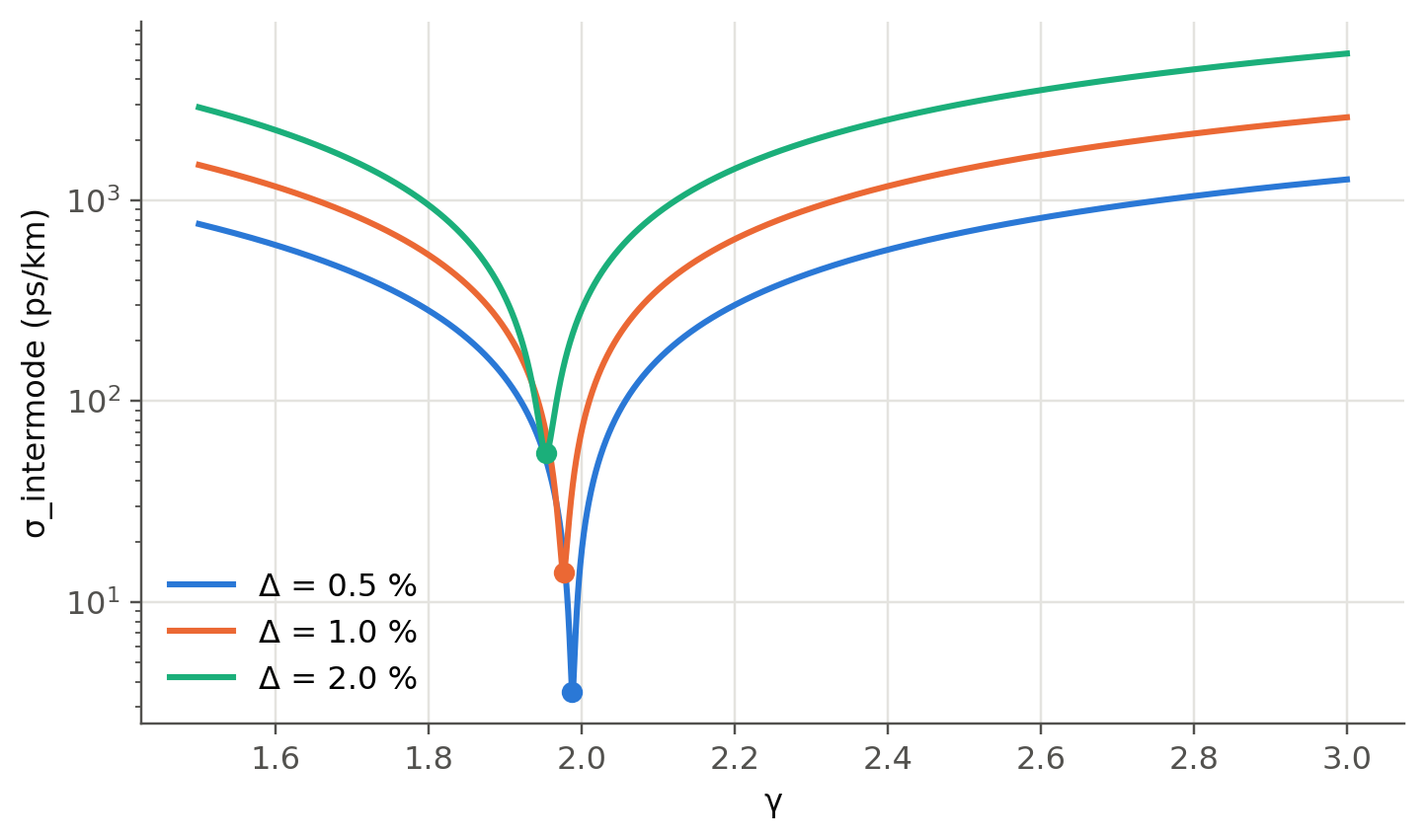
Wave theory gives the rms intermodal spread for any $\gamma$ (Olshansky & Keck). With no profile dispersion, it is
minimum at $\gamma_\text{opt}\approx2-\tfrac{12}{5}\Delta$, where
$$
\sigma_\text{intermode}\approx\frac{L\,n_1\Delta^2}{20\sqrt3\,c} .
$$
```{python}
#| label: fig-gamma
#| fig-cap: "rms intermodal spread per km versus profile index γ (n1 = 1.475). The minimum is extremely sharp. A 10–15 % error in γ costs an order of magnitude in bandwidth (slide 132)."
g = np.linspace(1.5, 3.0, 2000)
fig, ax = plt.subplots()
for k, D_ in enumerate([0.005, 0.01, 0.02]):
    s = fl.sigma_intermodal_grin(g, 1.475, D_) * 1e12
    ax.semilogy(g, s, color=fl.PALETTE[k], label=f"Δ = {D_*100:.1f} %")
    i = s.argmin(); ax.plot(g[i], s[i], "o", color=fl.PALETTE[k])
    print(f"Δ = {D_:.3f}: γ_opt = {g[i]:.4f} (2 − 12Δ/5 = {2-12*D_/5:.4f}), σ_min = {s[i]:.2f} ps/km "
          f"(formula {1.475*D_**2/(20*np.sqrt(3)*c0)*1e15:.2f}), σ at 1.15γ_opt = {fl.sigma_intermodal_grin(1.15*g[i],1.475,D_)*1e12:.0f} ps/km")
ax.set_xlabel("γ"); ax.set_ylabel("σ_intermode (ps/km)"); ax.legend()
plt.show()
```
## Worked examples, recomputed
```{python}
c = c0
# Slides 128-131 : 50 µm GRIN, n1 = 1.475, Δ = 0.01, 850 nm VCSEL 0.4 nm, Dch = -100 ps/nm/km
n1, D_ = 1.475, 0.01
n2 = n1 * (1 - D_)
V = fl.V_number(25e-6, 0.85e-6, n1, n2)
sig_inter = n1 * D_**2 / (20 * np.sqrt(3) * c) * 1e3          # s over 1 km
t_inter = np.sqrt(6) * sig_inter                             # FWHM, triangular pulse
t_intra = 100e-12 * 0.4                                      # FWHM
t_tot = np.hypot(t_inter, t_intra)
sig_tot = t_tot / np.sqrt(6)        # triangular-pulse rms
B = 0.25 / sig_tot
print(f"Slides 128–131: n2 = {n2:.4f}, V = {V:.2f}, M ≈ V²/4 = {V**2/4:.0f}")
print(f"  σ_inter = {sig_inter*1e12:.2f} ps/km, τ_inter = {t_inter*1e12:.1f} ps, τ_intra = {t_intra*1e12:.1f} ps, "
      f"τ = {t_tot*1e12:.1f} ps → B = 0.25/σ ≈ {B/1e9:.1f} Gb/s, f_op ≈ 0.99B = {0.99*B/1e9:.1f} GHz")
step = (n1 - n2) / c * 1e3
print(f"  same indices, step-index: Δτ ≈ {step*1e9:.1f} ns/km → BL ≈ 0.25/(0.29Δτ) = {0.25/(0.29*step)/1e6:.1f} Mb/s·km")

# Slide 132
n1, n2 = 1.48, 1.46; D_ = (n1 - n2) / n1
s = n1 * D_**2 / (20 * np.sqrt(3) * c) * 1e3
print(f"\nSlide 132: Δ = {D_:.4f}, σ = {s*1e9:.3f} ns/km, BL = {0.25/s/1e9:.1f} Gb/s·km; "
      f"step: {(n1-n2)/c*1e12:.1f} ns/km, BL = {0.25/(0.29*(n1-n2)/c*1e3)/1e6:.1f} Mb/s·km")

# Slide 133 : combining intermodal and intramodal
n1, n2 = 1.474, 1.453; D_ = (n1 - n2) / n1
s_inter = n1 * D_**2 / (20 * np.sqrt(3) * c) * 1e3
s_intra = 0.425 * 7.5e-12 * 3
s_tot = np.hypot(s_inter, s_intra)
print(f"\nSlide 133: Δ = {D_:.5f}, σ_inter = {s_inter*1e9:.4f} ns, σ_intra = {s_intra*1e9:.4f} ns, "
      f"σ = {s_tot*1e9:.4f} ns → B = {0.25/s_tot/1e9:.1f} Gb/s (L = 1 km)")
```
## GRIN rod lenses (slide 134)
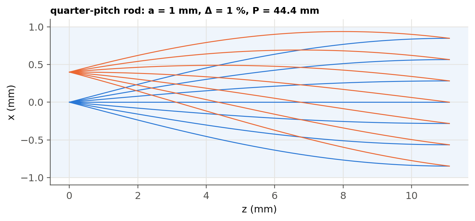
A parabolic rod ($\gamma=2$) with $n(r)\approx n_1[1-\tfrac{A}{2}r^2]$, $\sqrt A=\sqrt{2\Delta}/a$, makes every paraxial
ray oscillate with the same period, the **pitch** $P=2\pi/\sqrt A$. A quarter-pitch rod collimates a point source on
its face. A half-pitch rod images the front face onto the back face (inverted).
```{python}
#| label: fig-grinrod
#| fig-cap: "Rays from a point on the axis of a 0.25-pitch GRIN rod come out collimated. Rays from an off-axis point leave parallel to each other but tilted."
a_r, D_r = 1e-3, 0.01
P = 2 * np.pi * a_r / np.sqrt(2 * D_r)
z = np.linspace(0, 0.25 * P, 300); g_ = 2 * np.pi / P
fig, ax = plt.subplots(figsize=(8, 3.2))
ax.axhspan(-1, 1, color=fl.PALETTE[0], alpha=0.07, lw=0)
for x0, col in [(0, fl.PALETTE[0]), (0.4e-3, fl.PALETTE[1])]:
    for s0 in np.linspace(-0.12, 0.12, 7):
        x = x0 * np.cos(g_ * z) + s0 / g_ * np.sin(g_ * z)
        ax.plot(z * 1e3, x * 1e3, color=col, lw=1)
ax.set_xlabel("z (mm)"); ax.set_ylabel("x (mm)")
ax.set_title(f"quarter-pitch rod: a = 1 mm, Δ = 1 %, P = {P*1e3:.1f} mm", loc="left", fontsize=10)
plt.show()
```
## Try it yourself
1. Add **profile dispersion** ($\varepsilon\neq0$ in `fl.sigma_intermodal_grin`): $\Delta$ itself depends on $\lambda$.
Show that a fiber optimised at 850 nm is no longer optimal at 1300 nm. This is why OM3/OM4 fibers are
specified at 850 nm (slide 127).
2. Launch **skew rays** in the ray tracer (3-D, conserve the angular momentum $n r^2 d\phi/ds$). Do they also arrive on time?
3. Compute the number of modes $M\approx\frac{\gamma}{\gamma+2}\frac{V^2}{2}$ and compare step ($\gamma\to\infty$) and parabolic.