1  Planar dielectric waveguides

 Run this chapter’s code in Google Colab (no installation).

Slides 7–39. A core of index \(n_1\) and thickness \(2a\) sandwiched between two claddings of index \(n_2<n_1\). It is the simplest waveguide, and almost everything we will say about fibers already appears here: modes, cut-off, the \(V\)-number, evanescent tails and dispersion.

1.1 The waveguide condition

A ray zig-zagging at angle \(\theta\) (from the normal) must interfere constructively with itself after two reflections (slides 9–11). With \(k_1=2\pi n_1/\lambda\) and a phase change \(\phi\) at each total internal reflection (TIR):

\[ \frac{2\pi n_1 (2a)}{\lambda}\cos\theta_m-\phi_m=m\pi ,\qquad m=0,1,2,\dots \tag{1.1}\]

The TIR phase for TE (E along \(x\), perpendicular to the plane of incidence) and TM polarisation is

\[ \tan\frac{\phi_m}{2}=\frac{\sqrt{\sin^2\theta_m-(n_2/n_1)^2}}{\cos\theta_m}\;(\text{TE}),\qquad \tan\frac{\phi_m}{2}=\frac{\sqrt{\sin^2\theta_m-(n_2/n_1)^2}}{(n_2/n_1)^2\cos\theta_m}\;(\text{TM}). \]

Each allowed angle \(\theta_m\) is a mode. Its propagation constant along the guide is \(\beta_m=k_1\sin\theta_m\), and the transverse one is \(\kappa_m=k_1\cos\theta_m\) (slide 12). We can write \(\beta_m = k_0 n_\text{eff}\) with \(n_2<n_\text{eff}=n_1\sin\theta_m<n_1\).

1.1.1 Graphical solution, live

Introduce \(u=k_1 a\cos\theta\) and \(w=a\sqrt{\beta^2-k_0^2n_2^2}\). Then \(u^2+w^2=V^2\), and Equation 1.1 becomes the classic pair (TE):

\[ w = u\tan u \;\;(\text{even modes } m=0,2,\dots),\qquad w = -u\cot u \;\;(\text{odd modes } m=1,3,\dots). \]

The guided modes are the intersections of these curves with the circle of radius \(V\). Move the slider: a new mode appears each time \(V\) crosses a multiple of \(\pi/2\).

viewof Vslab = Inputs.range([0.2, 12], {value: 3.15, step: 0.01, label: "V-number"})

slabCurves = {
  const pts = [];
  for (let k = 0; k < 9; k++) {           // branches of u tan u and -u cot u
    const u0 = k * Math.PI / 2, even = k % 2 === 0;
    for (let i = 1; i < 400; i++) {
      const u = u0 + (Math.PI / 2) * i / 400;
      const w = even ? u * Math.tan(u) : -u / Math.tan(u);
      if (w >= 0 && w < 14) pts.push({u, w, branch: k, parity: even ? "even (u tan u)" : "odd (−u cot u)"});
    }
  }
  return pts;
}
slabRoots = {
  const out = [];
  for (let k = 0; k * Math.PI / 2 < Vslab; k++) {
    const even = k % 2 === 0;
    const f = u => (even ? u * Math.tan(u) : -u / Math.tan(u)) - Math.sqrt(Math.max(Vslab*Vslab - u*u, 0));
    let lo = k * Math.PI / 2 + 1e-9, hi = Math.min((k + 1) * Math.PI / 2 - 1e-9, Vslab);
    for (let it = 0; it < 80; it++) { const mid = (lo + hi) / 2; (f(lo) * f(mid) <= 0) ? hi = mid : lo = mid; }
    const u = (lo + hi) / 2;
    out.push({m: k, u, w: Math.sqrt(Math.max(Vslab*Vslab - u*u, 0)), b: 1 - (u/Vslab)**2});
  }
  return out;
}
Plot.plot({
  width: 640, height: 380, x: {label: "u = k₁a cos θ", domain: [0, 12.5]}, y: {label: "w", domain: [0, 12.5]},
  color: {domain: ["even (u tan u)", "odd (−u cot u)"], range: ["#2a78d6", "#eb6834"], legend: true},
  marks: [
    Plot.line(slabCurves, {x: "u", y: "w", z: "branch", stroke: "parity", strokeWidth: 2}),
    Plot.line(d3.range(0, 1.0001, 0.005).map(t => ({u: Vslab*Math.cos(t*Math.PI/2), w: Vslab*Math.sin(t*Math.PI/2)})),
              {x: "u", y: "w", stroke: "#52514e", strokeDasharray: "4,3"}),
    Plot.dot(slabRoots, {x: "u", y: "w", r: 6, fill: "#0b0b0b", stroke: "white", strokeWidth: 2, tip: true,
             title: d => `TE${d.m}\nu = ${d.u.toFixed(3)}\nw = ${d.w.toFixed(3)}\nb = ${d.b.toFixed(4)}`}),
    Plot.text(slabRoots, {x: "u", y: "w", text: d => `TE${d.m}`, dy: -14, fontWeight: "bold"}),
    Plot.ruleY([0]), Plot.ruleX([0])
  ]
})

html`<div class="result-box">V = ${Vslab.toFixed(2)} → <b>${slabRoots.length} TE mode(s)</b>
  (formula: M = ⌊2V/π⌋ + 1 = ${Math.floor(2*Vslab/Math.PI)+1}).
  ${Vslab < Math.PI/2 ? "Single-mode: V < π/2." : ""}</div>`

1.2 Worked example: the 20 µm guide (slides 24–26)

A planar guide with \(2a=20\) µm, \(n_1=1.455\), \(n_2=1.440\), \(\lambda=900\) nm. Find the modes.

d, wl, n1, n2 = 20e-6, 900e-9, 1.455, 1.440
th = fl.slab_modes(d, wl, n1, n2, "TE")
pen = fl.slab_penetration(th, wl, n1, n2)
V = fl.V_number(d / 2, wl, n1, n2)

import pandas as pd
tab = pd.DataFrame({"m": range(len(th)),
                    "θ_m (deg)": np.degrees(th).round(1),
                    "δ_m (µm)": (pen * 1e6).round(3),
                    "n_eff": (n1 * np.sin(th)).round(4)})
print(f"V = {V:.2f}, critical angle θc = {np.degrees(np.arcsin(n2/n1)):.2f}°, "
      f"number of TE modes = {len(th)} (TM: {len(fl.slab_modes(d, wl, n1, n2, 'TM'))})")
tab.style.hide(axis="index")

V = 14.55, critical angle θc = 81.77°, number of TE modes = 10 (TM: 10)

m	θ_m (deg)	δ_m (µm)	n_eff
0	89.200000	0.691000	1.454800
1	88.300000	0.702000	1.454400
2	87.500000	0.721000	1.453600
3	86.700000	0.751000	1.452600
4	85.900000	0.796000	1.451200
5	85.000000	0.862000	1.449600
6	84.200000	0.966000	1.447600
7	83.400000	1.146000	1.445400
8	82.600000	1.544000	1.443000
9	81.900000	3.864000	1.440500

The table reproduces slide 26 exactly. Notice two trends.

• Higher modes travel at steeper angles (smaller \(\theta_m\), closer to \(\theta_c\)).
• Higher modes have a larger penetration \(\delta_m\) into the cladding, and it diverges near cut-off.

1.2.1 Mode field patterns

Inside the core the field is a standing wave \(\cos(\kappa y)\) or \(\sin(\kappa y)\). In the cladding it decays as \(\exp(-|y|/\delta_m)\) (slides 16–20).

y = np.linspace(-18e-6, 18e-6, 1500)
fig, ax = plt.subplots(figsize=(8, 4))
ax.axvspan(-10, 10, color=fl.PALETTE[0], alpha=0.08, lw=0)
for k, m in enumerate([0, 1, 2, 9]):
    E = fl.slab_field(y, d, wl, n1, n2, th[m], m)
    ax.plot(y * 1e6, E + 2.4 * k, color=fl.PALETTE[k])
    ax.text(18.5, 2.4 * k, f"TE$_{m}$", va="center", color=fl.INK)
ax.set_xlabel("y (µm)"); ax.set_yticks([]); ax.set_xlim(-18, 20.5)
ax.set_title("Transverse field $E_m(y)$")
plt.show()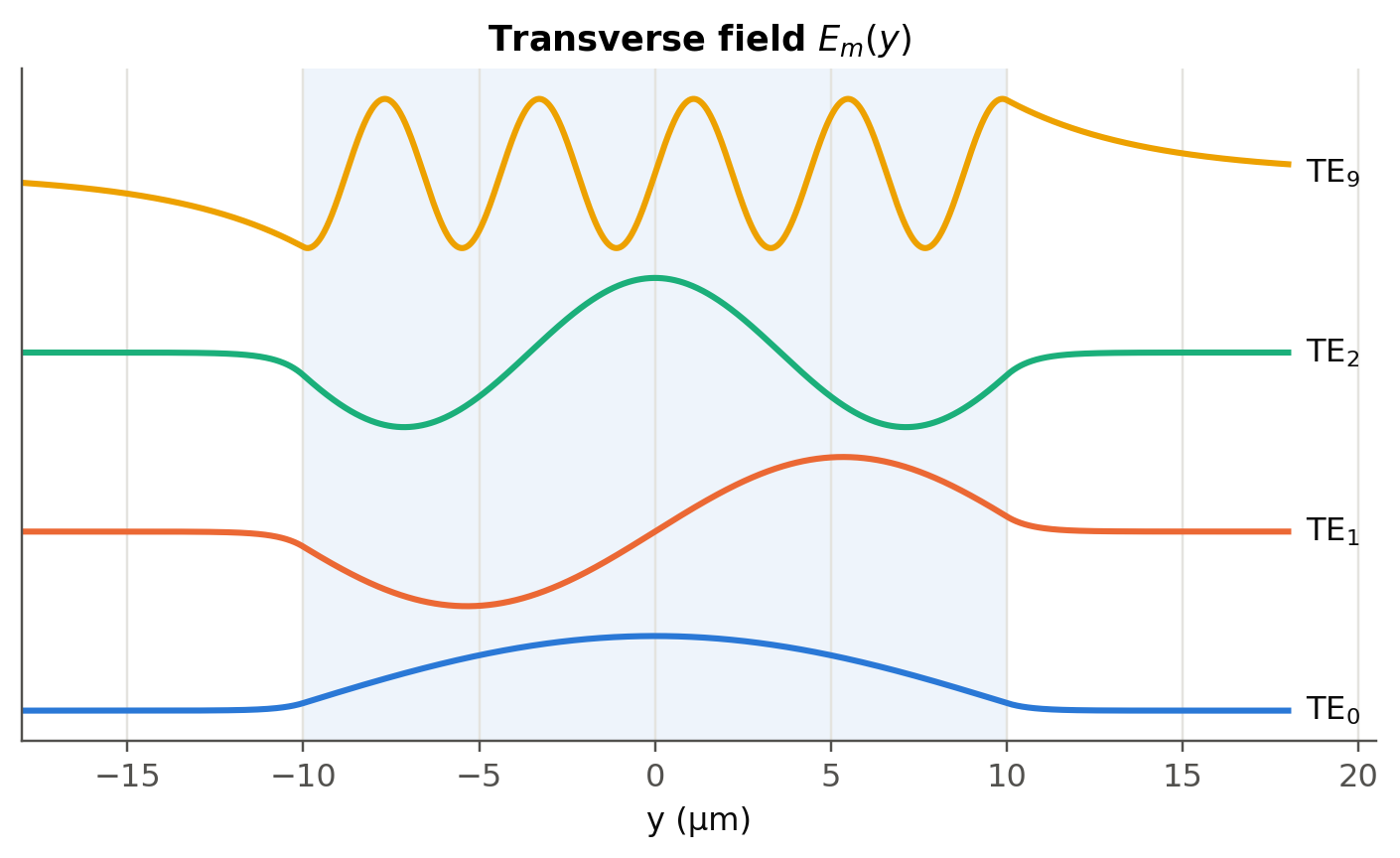

Figure 1.1: TE mode fields of the 20 µm guide at 900 nm. The shaded band is the core. Higher modes spill further into the cladding.

1.2.2 Mode field width (slide 29)

A semi-quantitative width is \(2w_0 = 2a + 2\delta\). For a single-mode slab this becomes \(2w_0 \approx 2a\,(V+1)/V\). We will see a more rigorous definition for fibers (MFD).

1.3 \(V\)-number and number of modes (slides 22, 28)

\[ V=\frac{2\pi a}{\lambda}\sqrt{n_1^2-n_2^2},\qquad M=\left\lfloor \frac{2V}{\pi}\right\rfloor+1 . \]

For \(V<\pi/2\) only TE\(_0\) (and TM\(_0\)) propagate. The cut-off wavelength is \(\lambda_c = 4a\sqrt{n_1^2-n_2^2}\). Above it the slab is single-mode.

wls = np.linspace(0.4e-6, 4e-6, 400)
counts = [len(fl.slab_modes(d, w, n1, n2)) for w in wls]
Vs = fl.V_number(d / 2, wls, n1, n2)
fig, ax = plt.subplots()
ax.step(wls * 1e6, counts, where="mid", label="exact count")
ax.plot(wls * 1e6, 2 * Vs / np.pi + 1, "--", color=fl.PALETTE[1], lw=1.5, label="2V/π + 1")
ax.set_xlabel("λ (µm)"); ax.set_ylabel("number of TE modes"); ax.legend()
lc = 4 * (d / 2) * np.sqrt(n1**2 - n2**2)
ax.axvline(lc * 1e6, color=fl.INK2, lw=1, ls=":")
ax.text(lc * 1e6, ax.get_ylim()[1] * 0.85, f"  λc = {lc*1e6:.2f} µm", color=fl.INK2)
plt.show()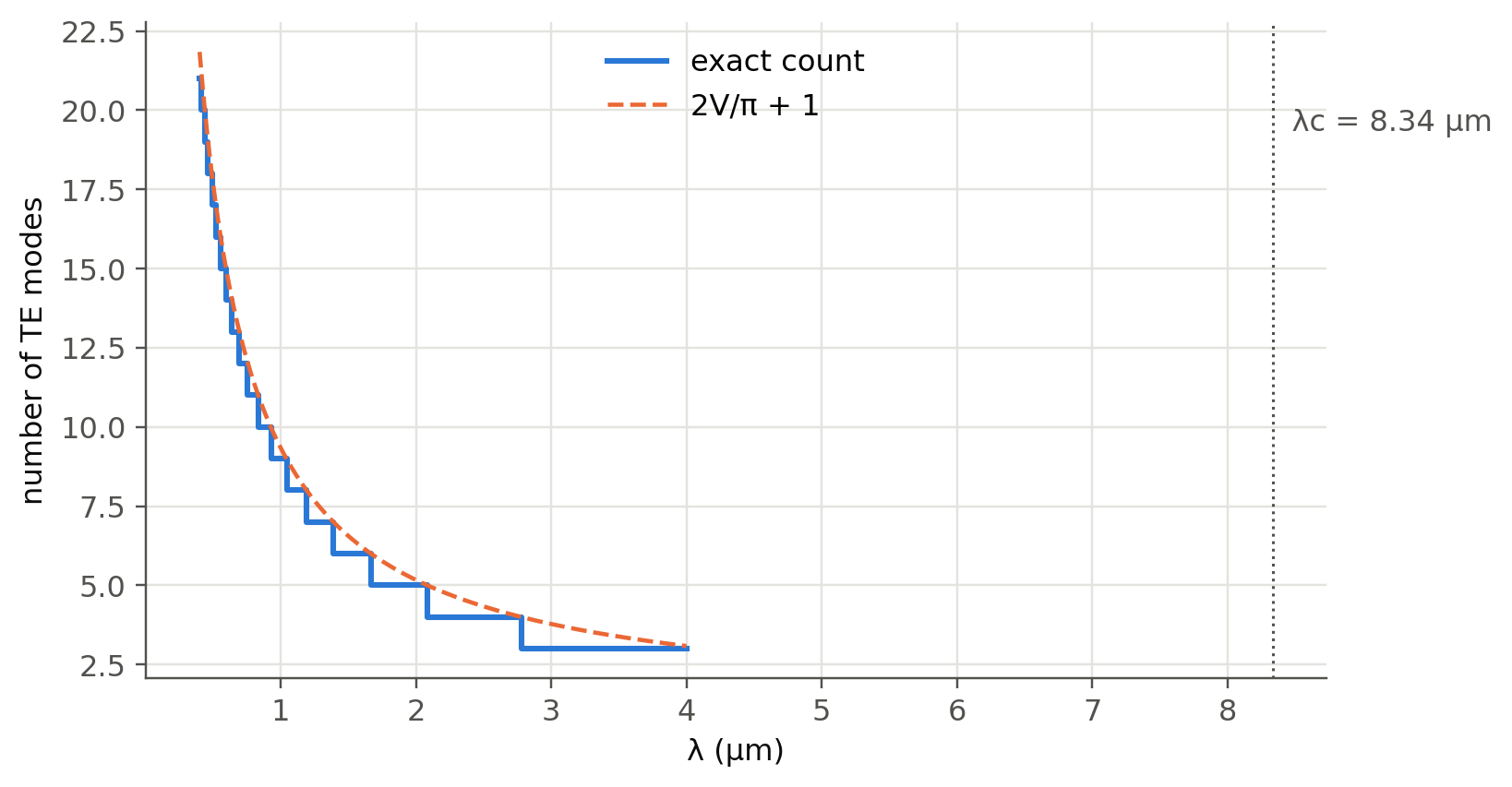

Figure 1.2: Number of TE modes versus wavelength for the 20 µm guide. The staircase follows 2V/π.

1.4 Dispersion diagram and group velocity (slides 30–39)

Each mode has its own \(\beta_m(\omega)\). The group velocity is the slope \(v_g = d\omega/d\beta\). Here we compute it exactly, with non-dispersive \(n_1\), \(n_2\) so that only the waveguide effect remains. These are the “calculations by the author” curves of slides 32–36.

def vg_curve(m, omegas):
    beta = np.array([fl.slab_beta(w, d, n1, n2, m) for w in omegas])
    return np.gradient(omegas, beta)

omegas = np.linspace(0.05e15, 1.6e16, 700)
fig, ax = plt.subplots(figsize=(8, 4.4))
for k, m in enumerate([0, 1, 4, 20, 40]):
    vg = vg_curve(m, omegas)
    ok = np.isfinite(vg)
    ax.plot(omegas[ok], vg[ok] / 1e8, color=fl.PALETTE[k], label=f"TE$_{{{m}}}$")
ax.axhline(c0 / n2 / 1e8, color=fl.INK2, ls=":", lw=1); ax.text(1.61e16, c0/n2/1e8, " c/n₂", va="center")
ax.axhline(c0 / n1 / 1e8, color=fl.INK2, ls=":", lw=1); ax.text(1.61e16, c0/n1/1e8, " c/n₁", va="center")
ax.axhline(c0 * n2 / n1**2 / 1e8, color=fl.INK2, ls="--", lw=1)
ax.text(1.61e16, c0*n2/n1**2/1e8, " (c/n₁)sinθc", va="center")
ax.set_xlabel("ω (rad/s)"); ax.set_ylabel("$v_g$ (×10⁸ m/s)"); ax.legend(ncol=5, loc="upper center")
ax.set_ylim(2.035, 2.09)
plt.show()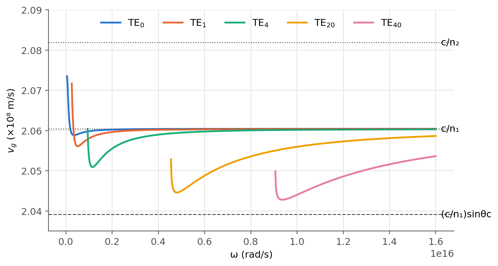

Figure 1.3: Group velocity of TE modes versus frequency (2a = 20 µm, n1 = 1.455, n2 = 1.440). Every mode starts at c/n2 at its cut-off, dips below c/n1 and tends to c/n1 at high frequency. Near cut-off a higher mode can be FASTER than TE0.

TipWhy can TE\(_1\) be faster than TE\(_0\)? (slide 38)

Near cut-off, a mode carries a large fraction of its power in the cladding, where light is faster (\(c/n_2\)). The ray picture (steeper ray means a longer path) is then not the whole story. The evanescent tail matters.

1.4.1 Intermodal dispersion of the slab

Far from cut-off the fastest mode travels at \(\approx c/n_1\) and the slowest at \(\approx (c/n_1)\sin\theta_c=c\,n_2/n_1^2\). The spread over a length \(L\) is therefore

\[ \frac{\Delta\tau}{L}\approx\frac{n_1-n_2}{c}\cdot\frac{n_1}{n_2}\approx\frac{n_1-n_2}{c}. \]

print(f"Δτ/L ≈ (n1-n2)/c = {(n1-n2)/c0*1e12*1e3/1e3:.1f} ps/m = {(n1-n2)/c0*1e9*1e3:.0f} ns/km")

Δτ/L ≈ (n1-n2)/c = 50.0 ps/m = 50 ns/km

At 50 ns/km a 1 ns pulse becomes 50 ns long after 1 km. This is why multimode guides are limited to short links.

1.5 Try it yourself

1. Use fl.slab_modes(..., "TM") and compare TE and TM angles. Which polarisation is more confined, and why (look at the \((n_2/n_1)^2\) factor)?
2. Find the thickness \(2a\) that makes the 20 µm-type guide single-mode at 1.55 µm.
3. Asymmetric slab (new): replace one cladding by air (\(n_3=1\)). The condition becomes \(2k_1a\cos\theta-\phi_{12}-\phi_{13}=2\pi m\). Write a 10-line solver and show that this guide has a non-zero cut-off even for the fundamental mode, unlike the symmetric one.
4. Compare with the online mode solver cited on slide 27 (computational-photonics.eu/oms.html).