# Projects and new ideas {#sec-ideas}
[](https://colab.research.google.com/github/{{< var github_user >}}/{{< var repo >}}/blob/main/{{< var subdir >}}/notebooks/ideas.ipynb){.colab-link} Run this chapter's code in Google Colab (no installation).
```{python}
#| include: false
import numpy as np
import matplotlib.pyplot as plt
import fiberlib as fl
fl.use_style()
c0 = fl.c0
```
This chapter collects **improvements to the course**, **topics that have become important since the slides were
written**, and **student projects** that reuse the code of this book.
## What has changed in fiber optics recently
| topic | why it matters | where it connects in Chapter 2 |
|---|---|---|
| **Coherent detection + DSP** | Chromatic dispersion and PMD are now undone digitally, so DCF disappears from new links | dispersion compensation, power fading |
| **Hollow-core anti-resonant fibers** | < 0.1 dB/km reported, 1/3 lower latency, ~1000× lower nonlinearity | special fibers, Rayleigh limit |
| **Space-division multiplexing** | multicore and few-mode fibers multiply capacity again (petabit/s per fiber in the lab) | LP modes, coupled-mode theory |
| **Multi-band (O to U)** | low-water-peak fibers + new amplifiers use > 50 nm beyond the C-band | attenuation spectrum, OH peak |
| **Distributed acoustic sensing on telecom cables** | φ-OTDR turns submarine and urban cables into seismometers and traffic sensors | OTDR, Rayleigh backscatter |
| **PAM-4 / IM-DD in data centres** | 100–200 Gb/s per lane over short SMF, close to λ₀ = 1310 nm | B²L limit, power fading |
| **Quantum key distribution** | single photons share fibers with classical channels, so Raman noise and FWM matter | nonlinear effects, Raman |
### A taste of the nonlinear Shannon limit
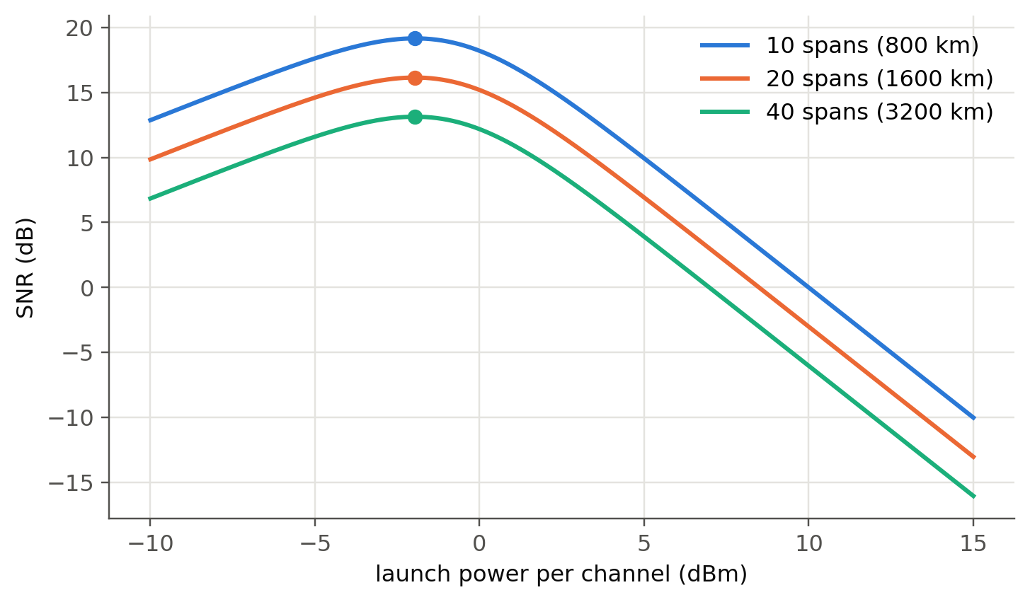
Amplified links add ASE noise ($\propto$ number of spans), and nonlinear interference grows as $P^3$ (the Gaussian-noise
model). The SNR, $\mathrm{SNR}=P/(P_\text{ASE}+\eta P^3)$, therefore has an **optimum launch power**, and the capacity
per fiber has a ceiling.
```{python}
#| label: fig-gn
#| fig-cap: "Toy GN-model: SNR versus launch power per channel for links of 10, 20 and 40 spans of 80 km. Below the optimum the link is noise-limited, above it nonlinearity-limited."
P = np.logspace(-4, -1.5, 300)          # W per channel
h_nu, NF, G = fl.h * 193.4e12, 10 ** 0.5, 10 ** (80 * 0.2 / 10)
B, eta1 = 32e9, 1.0e3                    # symbol bandwidth, NLI coefficient per span [1/W²]
fig, ax = plt.subplots()
for k, Ns in enumerate([10, 20, 40]):
    ase = Ns * NF * h_nu * G * B
    snr = P / (ase + Ns * eta1 * P**3)
    ax.plot(10 * np.log10(P / 1e-3), 10 * np.log10(snr), color=fl.PALETTE[k], label=f"{Ns} spans ({Ns*80} km)")
    i = snr.argmax(); ax.plot(10*np.log10(P[i]/1e-3), 10*np.log10(snr[i]), "o", color=fl.PALETTE[k])
ax.set_xlabel("launch power per channel (dBm)"); ax.set_ylabel("SNR (dB)"); ax.legend()
plt.show()
```
## Improvements to the course
1. **Live figures instead of screenshots.** Many slides show plots taken from books (b–V curves, $D(\lambda)$, loss
spectrum, eye diagrams). Every one of them is now regenerated in this book by a few lines of code. Students can change a
parameter and see the consequence, which builds intuition faster than a static picture.
2. **"Predict, then compute."** For each live panel, ask the class to predict the outcome before moving the slider
(e.g. *"What happens to the eye if D changes sign?"*). This is quick, engaging and well suited to peer instruction.
3. **Exercises with automatic checking.** The worked examples are all reproduced numerically, so they can become
exercises with randomised numbers (e.g. with [quarto-live](https://r-wasm.github.io/quarto-live/) or Pyodide, Python runs
in the browser and the answer can be checked on the spot). The problem set `Chapter2_Questions_Problems.pdf` is a natural
source.
4. **One running example through the chapter.** Use the same standard SMF (a = 4.1 µm, 3.5 % GeO₂) from modes → MFD →
dispersion → bend loss → link budget → eye diagram. Students then see how the design choices are coupled (e.g. a
smaller core shifts λ₀ but raises bend loss).
5. **Connect with the online link simulator** already used in the course
(see `opticallinksimulator.txt`) and with the in-browser simulator of @sec-bitrate.
6. **Shorten the sensor part, deepen the "why".** The gyroscope history slides (301–309) could become a single
timeline, freeing time for the Sagnac calculation and the OTDR trade-offs, which are more transferable skills.
## Student projects
Each project reuses `fiberlib.py` and can be done in 1–3 weeks.
| # | project | skills | difficulty |
|---|---|---|---|
| 1 | **Fiber design optimiser**: find (a, Δ) that give λ₀ = 1450 nm, single-mode above 1260 nm, MFD > 8.5 µm, and minimum bend loss | optimisation, mode solver | ★★ |
| 2 | **Three-layer (W / trench) fiber solver**: extend `LP_b` to a depressed cladding and reproduce a dispersion-flattened fiber | Bessel functions, root finding | ★★★ |
| 3 | **Split-step Fourier propagation**: SPM, soliton, and the GN-model optimum launch power | FFT, NLSE | ★★★ |
| 4 | **Chirped FBG dispersion compensator**: design a grating that compensates 80 km of SMF | TMM, group delay | ★★ |
| 5 | **OTDR event detector**: automatic detection/classification of events in a measured trace (least-squares, change-point, or a small ML classifier) | signal processing | ★★ |
| 6 | **PAM-4 vs NRZ data-centre link** at 1310 nm with `imdd_link` | modulation, BER | ★★ |
| 7 | **Few-mode fiber MDM**: LP-mode overlaps and mode-dependent loss; how many channels can a few-mode fiber carry? | modes, overlaps | ★★★ |
| 8 | **Raman DTS design**: required averaging for 1 K resolution at 10 km | noise, statistics | ★★ |
| 9 | **Measure your own fiber**: cut-back loss and bend loss with a lab source and power meter, compared with the models of @sec-attenuation | experiment | ★ |
## Useful open-source tools
- [OptiCommPy](https://github.com/edsonportosilva/OptiCommPy): transmitters, channels, DSP and coherent receivers in Python.
- [ofiber](https://github.com/scottprahl/ofiber) (S. Prahl): the package used in `ofiber_test.ipynb`. It is a good cross-check for
`fiberlib` (install with `pip install ofiber`).
- [GNPy](https://github.com/Telecominfraproject/oopt-gnpy): GN-model planning of real optical networks.
- [femwell](https://github.com/HelgeGehring/femwell), [Meep / MPB](https://meep.readthedocs.io): finite-element and FDTD solvers
for arbitrary waveguide cross-sections (PCF, multicore).
## Notes for the instructor: checks on the slides
While recomputing the examples, everything matched the slides except the following points, which deserve a second look:
- **Slide 222 (FBG):** the bandwidth formula $\frac{\lambda_B^2}{\pi nL}\sqrt{(\kappa L)^2+\pi^2}$ gives ≈ 0.20 nm, not 0.428 nm.
The periodicity uses $n=1.450$ while the statement gives $n_\text{eff}=1.4550$ (532.6 nm vs 534.5 nm).
- **Slide 146:** $0.90/1.55^4=0.156$ dB/km rather than 0.178 dB/km (the total would be 0.176 dB/km). The NA-based
value, 0.159 dB/km, is correct.
- **Slide 139 (Rayleigh):** the intermediate value is written both as $3.276\times10^{-2}$ and $3.735\times10^{-2}$ km⁻¹. The
correct one is $3.276\times10^{-2}$ km⁻¹, which gives 0.142 dB/km.
- **`opticomm.ipynb`:** the errors come from an API change in OptiCommPy ≥ 0.10 (`pulseShape` now takes a `parameters`
object, and `bsp` returns a different shape). A corrected cell is given in @sec-bitrate.
- **`ofiber_test.ipynb`** needs `pip install ofiber`. All of its plots have an equivalent in this book that does not depend on it.