# Fiber sensors: OTDR, distributed sensing, interferometers {#sec-sensors}
[](https://colab.research.google.com/github/{{< var github_user >}}/{{< var repo >}}/blob/main/{{< var subdir >}}/notebooks/sensors.ipynb){.colab-link} Run this chapter's code in Google Colab (no installation).
```{python}
#| include: false
import numpy as np
import matplotlib.pyplot as plt
import fiberlib as fl
fl.use_style()
c0 = fl.c0
```
*Slides 231–311.* The weaknesses of a fiber for telecom (scattering, sensitivity to strain and temperature) become
strengths for sensing. Fiber sensors are immune to EMI, need no electrical power at the sensing point, survive harsh
environments, and can be **distributed** along tens of km.
## Optical time-domain reflectometry (slides 245–266)
Send a short pulse and listen to the Rayleigh **backscatter**. Light returning at time $t$ comes from
$$
z=\frac{v_g t}{2},\qquad \Delta z_\text{res}=\frac{v_g\tau}{2}\ (\text{pulse width }\tau).
$$
The backscattered power from position $z$ is
$$
P_{bs}(z)=P_0\,S\,\alpha_s\,\frac{v_g\tau}{2}\,e^{-2\alpha z},
$$
where $S\approx10^{-3}$ is the capture factor and $\alpha_s$ the scattering coefficient. OTDR traces are plotted in
**one-way dB**, $5\log_{10}P$, so that the slope reads directly as the fiber attenuation.
### Example (slide 262)
```{python}
P0 = fl.dBm_to_W(13); tau = 10e-6; vg = c0 / 1.468
alpha = 0.33 / 4.343 / 1e3; alpha_s = 0.3 / 4.343 / 1e3; S = 1e-3
for z in [0, 50e3, 100e3]:
    P = P0 * S * alpha_s * vg * tau / 2 * np.exp(-2 * alpha * z)
    print(f"z = {z/1e3:5.0f} km:  P_bs = {P*1e9:9.3f} nW = {fl.W_to_dBm(P):6.1f} dBm")
print(f"Spatial resolution with τ = 10 µs: {vg*tau/2:.0f} m")
```
### Averaging (slides 252–253)
Noise falls as $\sqrt N$ with $N$ averaged shots. Each shot must wait one round trip, $T=2nL/c$.
```{python}
L = 10e3; T = 2 * 1.468 * L / c0
for t_meas in [1, 180]:
    N = 0.9 * t_meas / T
    print(f"{t_meas:4d} s: N = {N:.3g} shots → noise reduced by √N = {np.sqrt(N):.0f}× "
          f"= {5*np.log10(N):.1f} dB (one-way OTDR scale)")
```
### OTDR simulator, live
The fiber below has a front connector, a fusion splice at 8 km, a tight bend at 15 km, a mechanical splice at 22 km
and an open end at 30 km. Change the pulse width and the averaging, and look at the trade-off between **dynamic range**
and **resolution** (slide 256).
```{ojs}
//| echo: false
viewof ot = Inputs.form({
  tau: Inputs.select([10, 30, 100, 300, 1000, 3000, 10000], {value: 300, label: "pulse width (ns)"}),
  N:   Inputs.select([1, 16, 256, 4096, 65536], {value: 256, label: "averages"}),
  a:   Inputs.range([0.15, 0.5], {value: 0.33, step: 0.01, label: "loss (dB/km)"})
})
```
```{ojs}
//| echo: false
otdr = {
  const dz = 2, Lmax = 34000, vg = 299792458 / 1.468, W = vg * ot.tau * 1e-9 / 2;   // m
  const n = Math.floor(Lmax / dz);
  const events = [{z: 8000, loss: 0.1, refl: 0}, {z: 15000, loss: 0.6, refl: 0},
                  {z: 22000, loss: 0.4, refl: 1e-4}, {z: 30000, loss: 99, refl: 0.035}];
  const a = ot.a / 4.343 / 1000, as = 0.3 / 4.343 / 1000;
  const raw = new Float64Array(n); let lossdB = 0;
  for (let i = 0; i < n; i++) {
    const z = i * dz;
    for (const e of events) if (z >= e.z && z - dz < e.z) { raw[i] += e.refl / dz * 10 ** (-lossdB / 5); lossdB += e.loss; }
    if (lossdB < 50) raw[i] += 1e-3 * as * 10 ** (-lossdB / 5) * Math.exp(-2 * a * z);
  }
  const k = Math.max(1, Math.round(W / dz)), conv = new Float64Array(n); let acc = 0;   // rectangular pulse
  for (let i = 0; i < n; i++) { acc += raw[i]; if (i >= k) acc -= raw[i - k]; conv[i] = acc * dz; }
  const P0 = 0.02, noise = 3e-12 / Math.sqrt(ot.N);              // W, receiver noise after averaging
  const out = [];
  for (let i = 0; i < n; i += 5) {
    const u1 = Math.random() || 1e-12, u2 = Math.random();
    const p = P0 * conv[i] + noise * Math.sqrt(-2 * Math.log(u1)) * Math.cos(2 * Math.PI * u2);
    out.push({z: i * dz / 1000, dB: 5 * Math.log10(Math.max(p, 1e-16) / 1e-3)});
  }
  const p0 = 5 * Math.log10(P0 * 1e-3 * as * W / 1e-3), floor = 5 * Math.log10(noise / 1e-3);
  return {out, W, DR: p0 - floor, floor};
}
Plot.plot({
  width: Math.min(width, 1050), height: 340, x: {label: "distance (km)"}, y: {label: "backscatter (dB, one-way, rel. 1 mW)", grid: true},
  marks: [Plot.line(otdr.out, {x: "z", y: "dB", stroke: "#2a78d6", strokeWidth: 1.2}),
          Plot.ruleY([otdr.floor], {stroke: "#e34948", strokeDasharray: "4,3"}),
          Plot.text(["fusion splice", "bend", "mech. splice", "end"], {x: [8, 15, 22, 30], y: otdr.floor + 2, dy: -6, fill: "#52514e", fontSize: 10})]
})
```
```{ojs}
//| echo: false
html`<div class="result-box">pulse ${ot.tau} ns → spatial resolution ≈ <b>${otdr.W.toFixed(1)} m</b> ·
dynamic range ≈ <b>${otdr.DR.toFixed(1)} dB</b> (one-way) · red: noise floor after ${ot.N} averages</div>`
```
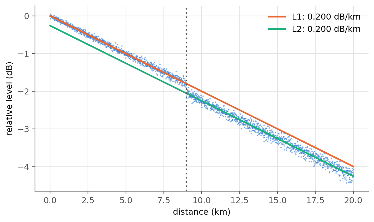
### Measuring a splice by least squares (slides 263–265)
```{python}
#| label: fig-splice
#| fig-cap: "A splice loss is measured by fitting straight lines to the backscatter before and after the event and taking their vertical offset at the event position."
rng = np.random.default_rng(2)
z = np.linspace(0, 20, 2000)
true_loss, zs = 0.25, 9.0
y = -0.2 * z - true_loss * (z > zs) + rng.normal(0, 0.03 + 0.004 * z, z.size)
m1 = (z > 1) & (z < zs - 0.3); m2 = (z > zs + 0.3) & (z < 19)
p1, p2 = np.polyfit(z[m1], y[m1], 1), np.polyfit(z[m2], y[m2], 1)
fig, ax = plt.subplots()
ax.plot(z, y, ".", ms=1.5, color=fl.PALETTE[0], alpha=0.5)
ax.plot(z, np.polyval(p1, z), color=fl.PALETTE[1], label=f"L1: {-p1[0]:.3f} dB/km")
ax.plot(z, np.polyval(p2, z), color=fl.PALETTE[2], label=f"L2: {-p2[0]:.3f} dB/km")
ax.axvline(zs, color=fl.INK2, ls=":")
ax.set_xlabel("distance (km)"); ax.set_ylabel("relative level (dB)"); ax.legend()
plt.show()
print(f"Estimated splice loss = {np.polyval(p1, zs) - np.polyval(p2, zs):.3f} dB (true {true_loss} dB)")
```
## Raman distributed temperature sensing (slides 237–241)
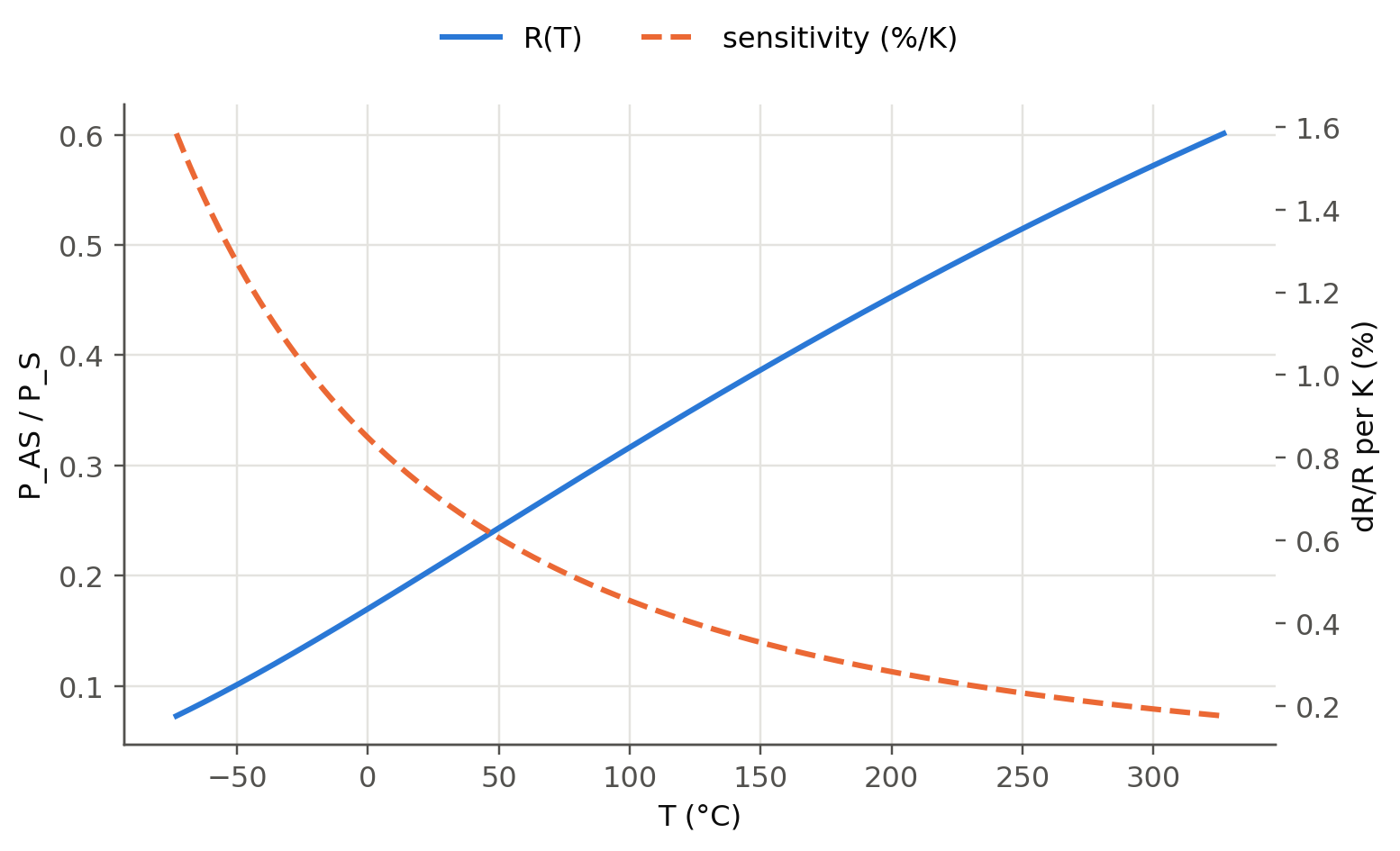
Spontaneous Raman scattering produces a Stokes and an anti-Stokes line shifted by ~13 THz. Only the anti-Stokes line
depends strongly on the phonon population, so their ratio is a thermometer:
$$
R(T)=\frac{P_{AS}}{P_S}=\left(\frac{\lambda_S}{\lambda_{AS}}\right)^4\exp\left(-\frac{h\Delta\nu}{k_BT}\right).
$$
```{python}
#| label: fig-raman
#| fig-cap: "Anti-Stokes/Stokes ratio versus temperature for a 1550 nm pump (Δν = 13.2 THz) and its relative sensitivity (≈ 0.8 %/K at room temperature)."
T = np.linspace(200, 600, 300)
dnu = 13.2e12; nu_p = c0 / 1550e-9
lS, lAS = c0 / (nu_p - dnu), c0 / (nu_p + dnu)
R = (lS / lAS) ** 4 * np.exp(-fl.h * dnu / (fl.kB * T))
fig, ax = plt.subplots()
ax.plot(T - 273.15, R, label="R(T)")
ax2 = ax.twinx(); ax2.grid(False)
ax2.plot(T - 273.15, 100 * fl.h * dnu / (fl.kB * T**2), "--", color=fl.PALETTE[1], label="sensitivity (%/K)")
ax.set_xlabel("T (°C)"); ax.set_ylabel("P_AS / P_S"); ax2.set_ylabel("dR/R per K (%)")
fig.legend(loc="upper center", ncol=2, frameon=False); plt.show()
print(f"Sensitivity at 25 °C: {100*fl.h*dnu/(fl.kB*298.15**2):.2f} %/K")
```
## Brillouin sensing (slides 242–244)
The backscattered Brillouin line is shifted by $\nu_B=2nv_a/\lambda$. Its shift depends on both strain and temperature.
```{python}
n, va = 1.45, 5960
for lam in [1.31e-6, 1.55e-6]:
    print(f"λ = {lam*1e6:.2f} µm: ν_B = {2*n*va/lam/1e9:.2f} GHz")
print("Typical coefficients in SMF at 1550 nm: ≈ 0.05 MHz/µε and ≈ 1.1 MHz/K, with a gain linewidth of ≈ 30 MHz.")
```
## Fabry–Perot filters and sensors (slides 271–283)
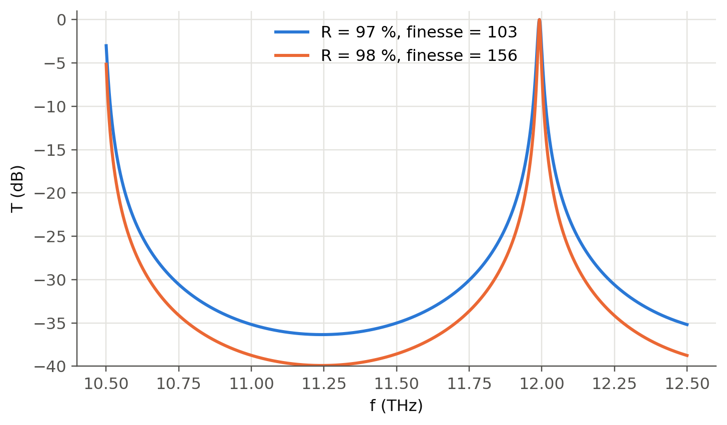
$$
T=\frac{1}{1+F\sin^2(\delta/2)},\qquad F=\frac{4R}{(1-R)^2},\qquad\delta=\frac{4\pi nd\nu}{c},\qquad
\mathrm{FSR}=\frac{c}{2nd},\qquad \mathcal F=\frac{\pi\sqrt R}{1-R}.
$$
```{python}
#| label: fig-fp
#| fig-cap: "Transmission of a Fabry–Perot filter with d = 100 µm (air), R = 97 % and 98 % (slide 277). The FSR is 1.5 THz. A higher R narrows the resonance and deepens the rejection."
nu = np.linspace(10.5e12, 12.5e12, 4000)
fig, ax = plt.subplots()
for k, R in enumerate([0.97, 0.98]):
    ax.plot(nu / 1e12, 10 * np.log10(fl.fabry_perot_T(nu, 100e-6, R)), color=fl.PALETTE[k],
            label=f"R = {R*100:.0f} %, finesse = {np.pi*np.sqrt(R)/(1-R):.0f}")
ax.set_xlabel("f (THz)"); ax.set_ylabel("T (dB)"); ax.set_ylim(-40, 1); ax.legend()
plt.show()
```
A change of the cavity length $\delta d$ (pressure on a diaphragm, strain, thermal expansion) shifts the fringes by
$\delta\nu/\nu=-\delta d/d$. This makes the Fabry–Perot one of the most sensitive point sensors (slides 279–283).
```{ojs}
//| echo: false
viewof fp = Inputs.form({
  R: Inputs.range([0.04, 0.995], {value: 0.9, step: 0.005, label: "mirror reflectance R"}),
  d: Inputs.range([10, 1000], {value: 100, step: 1, label: "gap d (µm)"}),
  dd: Inputs.range([-200, 200], {value: 0, step: 1, label: "displacement δd (nm)"})
})
```
```{ojs}
//| echo: false
{
  const F = 4 * fp.R / (1 - fp.R) ** 2, d = (fp.d + fp.dd * 1e-3) * 1e-6;
  const data = d3.range(1540, 1560, 0.005).map(l => {
    const dl = 4 * Math.PI * d / (l * 1e-9);
    return {l, T: 1 / (1 + F * Math.sin(dl / 2) ** 2)};
  });
  return Plot.plot({width: Math.min(width, 1050), height: 260, x: {label: "λ (nm)"}, y: {label: "transmission", domain: [0, 1.02]},
    marks: [Plot.line(data, {x: "l", y: "T", stroke: "#2a78d6", strokeWidth: 2})]});
}
```
```{ojs}
//| echo: false
html`<div class="result-box">FSR = ${(1550**2 / (2 * fp.d * 1000)).toFixed(2)} nm · finesse = ${(Math.PI * Math.sqrt(fp.R) / (1 - fp.R)).toFixed(1)} ·
fringe shift for δd = ${fp.dd} nm: ${(1550 * fp.dd * 1e-3 / fp.d).toFixed(3)} nm</div>`
```
## The Sagnac effect and fiber-optic gyroscopes (slides 284–311)
In a loop rotating at $\Omega$, the clockwise and counter-clockwise waves accumulate a phase difference
$$
\Delta\phi_S=\frac{2\pi LD}{\lambda c}\,\Omega=\frac{8\pi NA}{\lambda c}\,\Omega
$$
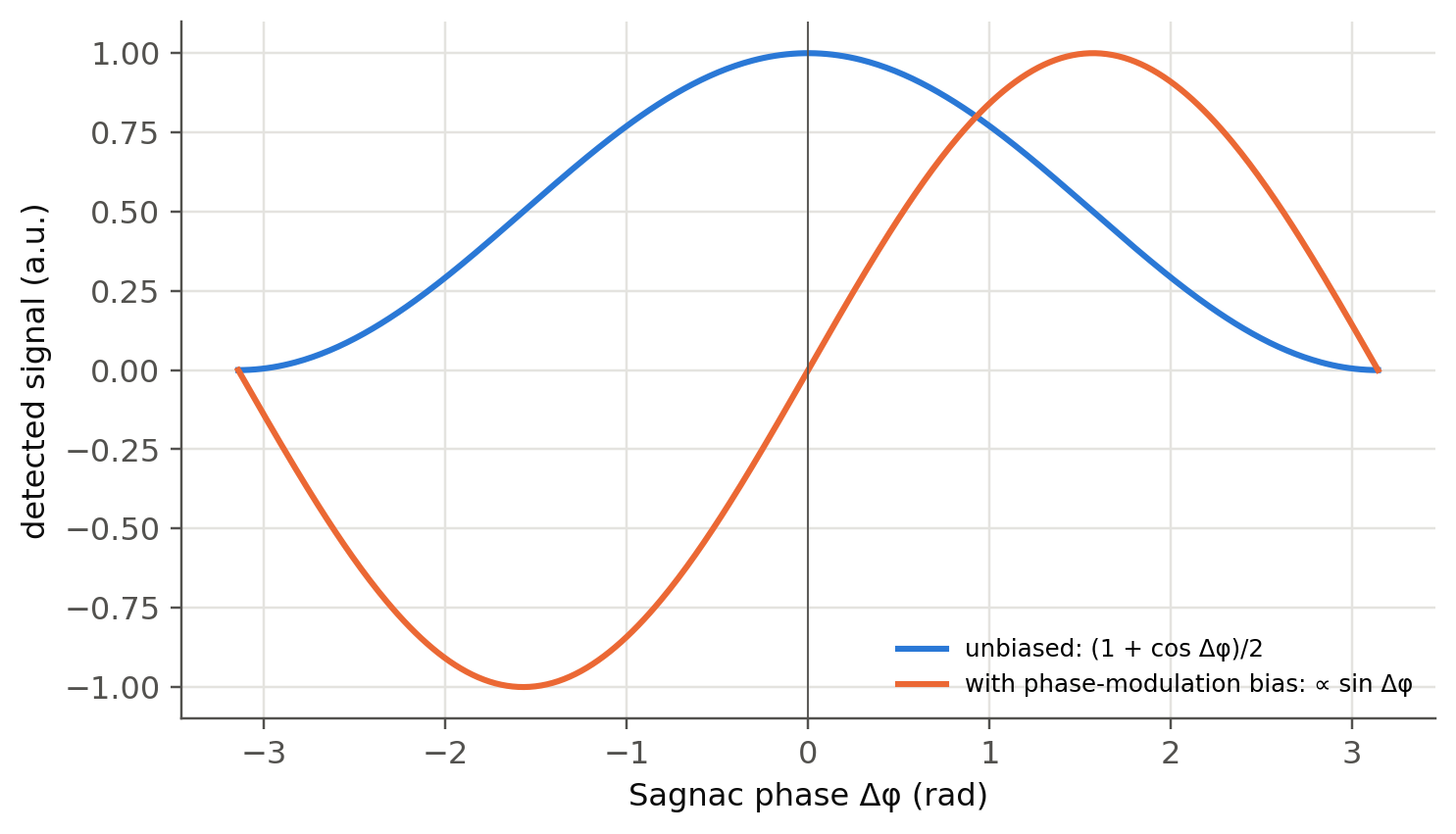
for a coil of length $L$ wound on a diameter $D$ (N turns of area A). Nothing else in the loop distinguishes the two
directions, so this tiny phase can be measured.
```{python}
#| label: fig-fog
#| fig-cap: "Open-loop FOG response. Without bias (cos response) the gyro is blind to small rotations and to their sign. A ±π/2 phase modulation turns the response into sin(Δφ), which is linear and signed around zero (slides 295–297)."
OmE = 7.292e-5                      # Earth rotation [rad/s]
for L, D in [(200, 0.03), (1000, 0.1), (5000, 0.2)]:
    print(f"L = {L:5d} m, D = {D*100:4.0f} cm: scale factor {2*np.pi*L*D/(1.55e-6*c0):.3f} rad/(rad/s), "
          f"Earth rotation → Δφ = {2*np.pi*L*D/(1.55e-6*c0)*OmE*1e6:.1f} µrad")
dphi = np.linspace(-np.pi, np.pi, 400)
fig, ax = plt.subplots()
ax.plot(dphi, (1 + np.cos(dphi)) / 2, label="unbiased: (1 + cos Δφ)/2")
ax.plot(dphi, np.sin(dphi), label="with phase-modulation bias: ∝ sin Δφ")
ax.axvline(0, color=fl.INK2, lw=0.6)
ax.set_xlabel("Sagnac phase Δφ (rad)"); ax.set_ylabel("detected signal (a.u.)"); ax.legend(fontsize=8)
plt.show()
```
## Try it yourself
1. Extend the OTDR simulator with a **reflective connector** and implement the **attenuation dead-zone** (receiver
saturation and recovery time).
2. A **φ-OTDR** (slide 267) uses a highly coherent laser: the backscatter becomes a speckle pattern whose changes reveal
vibrations. Simulate it by summing random-phase scatterers inside the pulse and perturbing the phase locally.
3. Compute the shot-noise-limited angle random walk of a FOG with 1 km coil, 100 µW at the detector. Compare with
tactical-grade (~0.1 °/√h) and navigation-grade (<0.001 °/√h) requirements.