# Dispersion {#sec-dispersion}
[](https://colab.research.google.com/github/{{< var github_user >}}/{{< var repo >}}/blob/main/{{< var subdir >}}/notebooks/dispersion.ipynb){.colab-link} Run this chapter's code in Google Colab (no installation).
```{python}
#| include: false
import numpy as np
import matplotlib.pyplot as plt
import fiberlib as fl
fl.use_style()
c0, PS = fl.c0, fl.PS_NM_KM
```
*Slides 65–95.* "Dispersion = spread of information." A short pulse that enters the fiber leaves it
broader, because its constituents (modes, wavelengths, polarisations) arrive at different times.
| mechanism | origin | where |
|---|---|---|
| intermodal | each mode has its own $v_g$ | MMF only |
| material | $n(\lambda)$, so $N_g(\lambda)$ | all fibers |
| waveguide | $v_g$ depends on $V(\lambda)$ | all fibers, tunable |
| profile | $\Delta(\lambda)$ | small, $<0.1$ ps nm$^{-1}$ km$^{-1}$ |
| polarisation (PMD) | random birefringence | SMF, grows as $\sqrt L$ |
| self-phase modulation | $n=n_0+n_2I$ | high power |
## Intermodal dispersion (slides 66–67)
Far from cut-off, the fastest and slowest rays differ by
$\Delta\tau/L\approx (n_1-n_2)/c=n_1\Delta/c$. The spread depends on length.
```{python}
for n1, n2 in [(1.48, 1.46), (1.475, 1.475*0.99), (1.4532, 1.4485)]:
    print(f"n1 = {n1:.4f}, n2 = {n2:.4f}:  Δτ/L ≈ {(n1-n2)/c0*1e12:.1f} ns/km")
```
## Chromatic dispersion in the fundamental mode (slides 68–71)
A source of spectral width $\Delta\lambda$ launches several wavelengths. Each has its own group delay
$\tau_g(\lambda)=L/v_g$. The **dispersion coefficient** is
$$
D=\frac1L\frac{d\tau_g}{d\lambda}\quad[\text{ps nm}^{-1}\text{km}^{-1}],\qquad
\Delta\tau = |D|\,L\,\Delta\lambda .
$$
### Material dispersion from the Sellmeier equation
$$
n^2(\lambda)=1+\sum_{i=1}^{3}\frac{B_i\lambda^2}{\lambda^2-\lambda_i^2},\qquad
N_g=n-\lambda\frac{dn}{d\lambda},\qquad
D_m=-\frac{\lambda}{c}\frac{d^2n}{d\lambda^2}.
$$
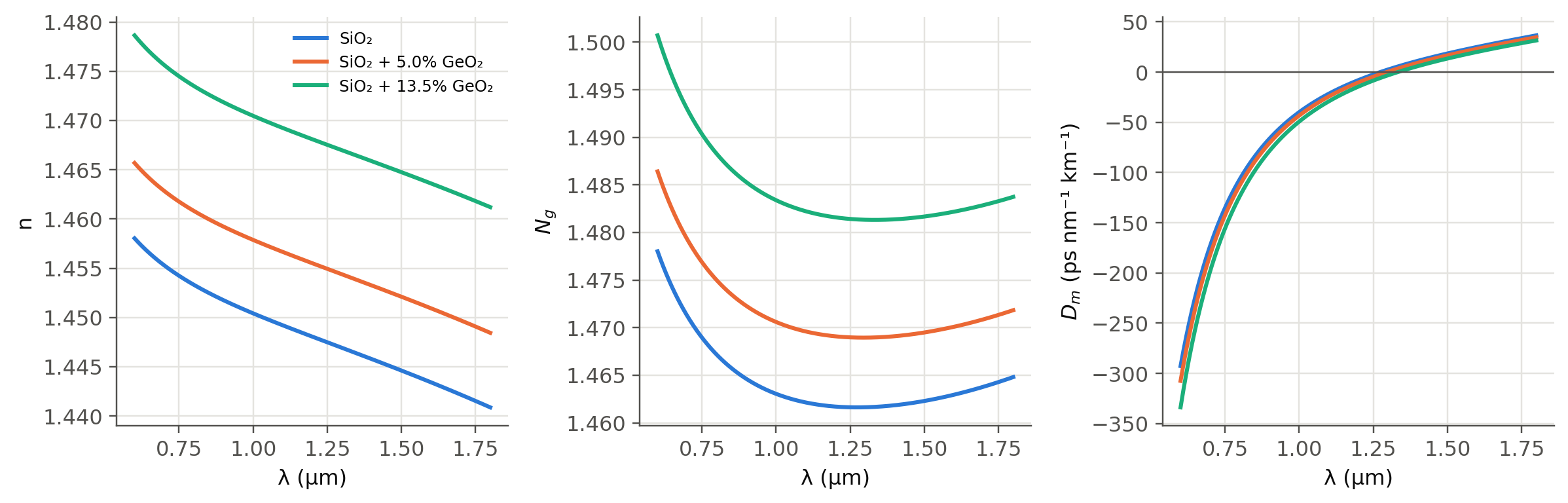
We use Malitson's coefficients for SiO$_2$ and Fleming's for GeO$_2$. A doped core
(SiO$_2$)$_{1-x}$(GeO$_2$)$_x$ is obtained by mixing the coefficients linearly.
```{python}
#| label: fig-sellmeier
#| fig-cap: "Refractive index n, group index Ng and material dispersion Dm of pure silica and germania-doped silica. Ng has a minimum where Dm crosses zero, near 1.27 µm for silica."
lam = np.linspace(0.6, 1.8, 500) * 1e-6
fig, axs = plt.subplots(1, 3, figsize=(11, 3.6))
for k, x in enumerate([0, 0.05, 0.135]):
    lab = "SiO₂" if x == 0 else f"SiO₂ + {x*100:.1f}% GeO₂"
    axs[0].plot(lam * 1e6, fl.n_doped(lam, x), color=fl.PALETTE[k], label=lab)
    axs[1].plot(lam * 1e6, fl.group_index(lam, x), color=fl.PALETTE[k])
    axs[2].plot(lam * 1e6, fl.D_material(lam, x) / PS, color=fl.PALETTE[k])
axs[0].set_ylabel("n"); axs[1].set_ylabel("$N_g$"); axs[2].set_ylabel("$D_m$ (ps nm⁻¹ km⁻¹)")
axs[2].axhline(0, color=fl.INK2, lw=0.8)
for ax in axs: ax.set_xlabel("λ (µm)")
axs[0].legend(fontsize=8)
plt.tight_layout(); plt.show()
from scipy.optimize import brentq
print("Zero material dispersion of silica: λ0 = %.1f nm" % (brentq(fl.D_material, 1.2e-6, 1.35e-6) * 1e9))
```
::: {.callout-tip}
## Positive and negative $D$ (slide 78)
$D>0$ means longer wavelengths arrive **later** ($N_g$ grows with $\lambda$). This is the "anomalous" regime
above 1.3 µm in silica. $D<0$ means shorter wavelengths arrive later. In fiber-optics jargon $D>0$ corresponds
to $\beta_2=-\lambda^2D/2\pi c<0$.
:::
### Waveguide dispersion (slides 74–76)
Even with constant $n_1, n_2$, the group delay depends on $\lambda$ through $V$:
$$
D_w\approx-\frac{n_2\Delta}{c\lambda}\,V\frac{d^2(Vb)}{dV^2},
\qquad V\frac{d^2(Vb)}{dV^2}\approx0.080+0.549(2.834-V)^2 .
$$
### Putting it together (slide 77)
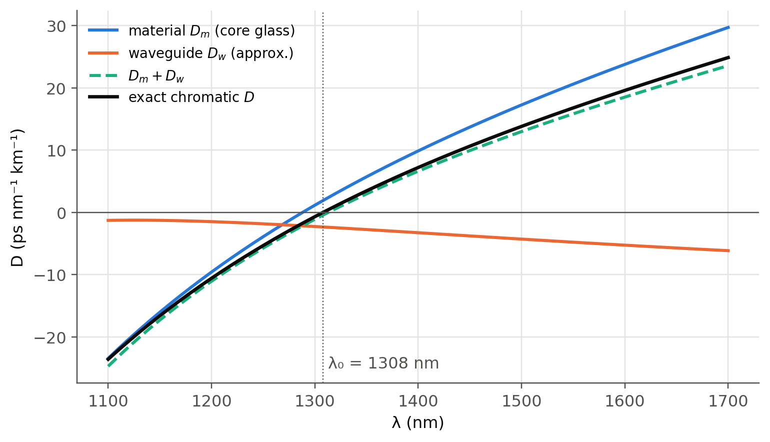
The "exact" chromatic dispersion follows from the effective index
$n_\text{eff}^2=n_2^2+b(V)(n_1^2-n_2^2)$ computed with the **wavelength-dependent** Sellmeier indices
and the **exact** $b(V)$. Then $\tau_g/L=(n_\text{eff}-\lambda\,dn_\text{eff}/d\lambda)/c$, and $D$ is its derivative.
This includes material, waveguide and profile dispersion at once, with no approximation beyond weak guidance.
```{python}
#| label: fig-chromatic
#| fig-cap: "Chromatic dispersion of a standard-like SMF (2a = 8.2 µm, core SiO2 + 3.5% GeO2, cladding SiO2). The exact result (black) matches Dm + Dw (approximation) closely and gives λ0 ≈ 1.31 µm and D ≈ 17 ps/nm/km at 1550 nm, like ITU-T G.652."
a, xc = 4.1e-6, 0.035
lam = np.linspace(1.1, 1.7, 61) * 1e-6
Dtot = np.array([fl.D_total_smf(l, a, xc) for l in lam]) / PS
Dm = fl.D_material(lam, xc) / PS
n2l = fl.n_silica(lam); n1l = fl.n_doped(lam, xc)
Dw = fl.D_waveguide_approx(lam, a, n2l, fl.Delta(n1l, n2l)) / PS
fig, ax = plt.subplots(figsize=(8, 4.4))
ax.plot(lam * 1e9, Dm, label="material $D_m$ (core glass)")
ax.plot(lam * 1e9, Dw, label="waveguide $D_w$ (approx.)")
ax.plot(lam * 1e9, Dm + Dw, "--", label="$D_m + D_w$")
ax.plot(lam * 1e9, Dtot, color=fl.INK, lw=2.2, label="exact chromatic $D$")
ax.axhline(0, color=fl.INK2, lw=0.8)
l0 = brentq(lambda l: fl.D_total_smf(l, a, xc), 1.25e-6, 1.4e-6)
ax.axvline(l0 * 1e9, color=fl.INK2, lw=0.8, ls=":")
ax.text(l0 * 1e9 + 5, -25, f"λ₀ = {l0*1e9:.0f} nm", color=fl.INK2)
ax.set_xlabel("λ (nm)"); ax.set_ylabel("D (ps nm⁻¹ km⁻¹)"); ax.legend(fontsize=9)
plt.show()
S0 = (fl.D_total_smf(l0 + 5e-9, a, xc) - fl.D_total_smf(l0 - 5e-9, a, xc)) / 10e-9 / PS * 1e-9
print(f"λ0 = {l0*1e9:.1f} nm, S0 = {S0:.3f} ps nm⁻² km⁻¹, D(1550) = {fl.D_total_smf(1.55e-6, a, xc)/PS:.2f} ps nm⁻¹ km⁻¹")
```
## Dispersion engineering, live (slides 76, 87–89)
$D_w$ is negative and grows in magnitude when the core gets **smaller** and the index step **larger**.
Pushing $\lambda_0$ to 1550 nm gives a *dispersion-shifted fiber* (DSF). Stopping slightly before gives a
*non-zero DSF* (NZ-DSF, G.655), which keeps a little dispersion to suppress four-wave mixing in WDM.
The curves below were computed with the exact model above. Pick a core radius and a GeO$_2$ concentration.
```{python}
#| echo: false
radii = np.round(np.arange(1.75, 5.01, 0.25), 2)
xs = [0.035, 0.05, 0.075, 0.10, 0.135]
lamg = np.linspace(1.15, 1.70, 23) * 1e-6
grid = {}
for a_ in radii:
for x_ in xs:
try:
grid[f"{a_:.2f}_{x_:.3f}"] = [float(fl.D_total_smf(l, a_ * 1e-6, x_) / PS) for l in lamg]
except Exception:
pass
ojs_define(dgrid={"lam": (lamg * 1e9).tolist(), "radii": radii.tolist(), "xs": xs, "D": grid})
```
```{ojs}
//| echo: false
viewof aSel = Inputs.select(dgrid.radii, {value: 4.0, label: "core radius a (µm)", format: d => d.toFixed(2)})
viewof xSel = Inputs.select(dgrid.xs, {value: 0.035, label: "GeO₂ mole fraction", format: d => (100*d).toFixed(1) + " %"})
```
```{ojs}
//| echo: false
dCurve = {
  const key = `${aSel.toFixed(2)}_${xSel.toFixed(3)}`;
  const D = dgrid.D[key] || [];
  return dgrid.lam.map((l, i) => ({lam: l, D: D[i]})).filter(d => Number.isFinite(d.D));
}
dRef = dgrid.lam.map((l, i) => ({lam: l, D: dgrid.D["4.00_0.035"][i]}))
dZero = {
  for (let i = 1; i < dCurve.length; i++) if (dCurve[i-1].D * dCurve[i].D <= 0) {
    const t = dCurve[i-1].D / (dCurve[i-1].D - dCurve[i].D);
    return dCurve[i-1].lam + t * (dCurve[i].lam - dCurve[i-1].lam);
  }
  return null;
}
Plot.plot({
  width: Math.min(width, 1050), height: 360, x: {label: "λ (nm)"}, y: {label: "D (ps nm⁻¹ km⁻¹)", domain: [-40, 30], grid: true},
  marks: [
    Plot.rectX([{x1: 1530, x2: 1565}], {x1: "x1", x2: "x2", fill: "#1baf7a", fillOpacity: 0.12}),
    Plot.text([{x: 1547, y: 27}], {x: "x", y: "y", text: () => "C-band", fill: "#52514e"}),
    Plot.ruleY([0], {stroke: "#52514e"}),
    Plot.line(dRef, {x: "lam", y: "D", stroke: "#b9b8b2", strokeDasharray: "4,3"}),
    Plot.line(dCurve, {x: "lam", y: "D", stroke: "#2a78d6", strokeWidth: 2.5}),
    Plot.dot(dCurve, {x: "lam", y: "D", r: 3, fill: "#2a78d6", tip: true,
             title: d => `λ = ${d.lam.toFixed(0)} nm\nD = ${d.D.toFixed(2)} ps/nm/km`})
  ]
})
```
```{ojs}
//| echo: false
{
  const D1550 = dCurve.length ? d3.scaleLinear().domain(dCurve.map(d => d.lam)).range(dCurve.map(d => d.D))(1550) : NaN;
  return html`<div class="result-box">a = ${aSel} µm, GeO₂ = ${(100*xSel).toFixed(1)} % ·
  λ₀ = ${dZero ? dZero.toFixed(0) + " nm" : "none in range"} · D(1550 nm) ≈ ${D1550.toFixed(1)} ps nm⁻¹ km⁻¹ ·
  dashed: standard SMF (a = 4 µm, 3.5 %).<br>
  <i>Watch out:</i> small cores shift λ₀ but also lower V. Check the single-mode cut-off and the bend loss!</div>`
}
```
## Commercial fibers (slides 90–92)
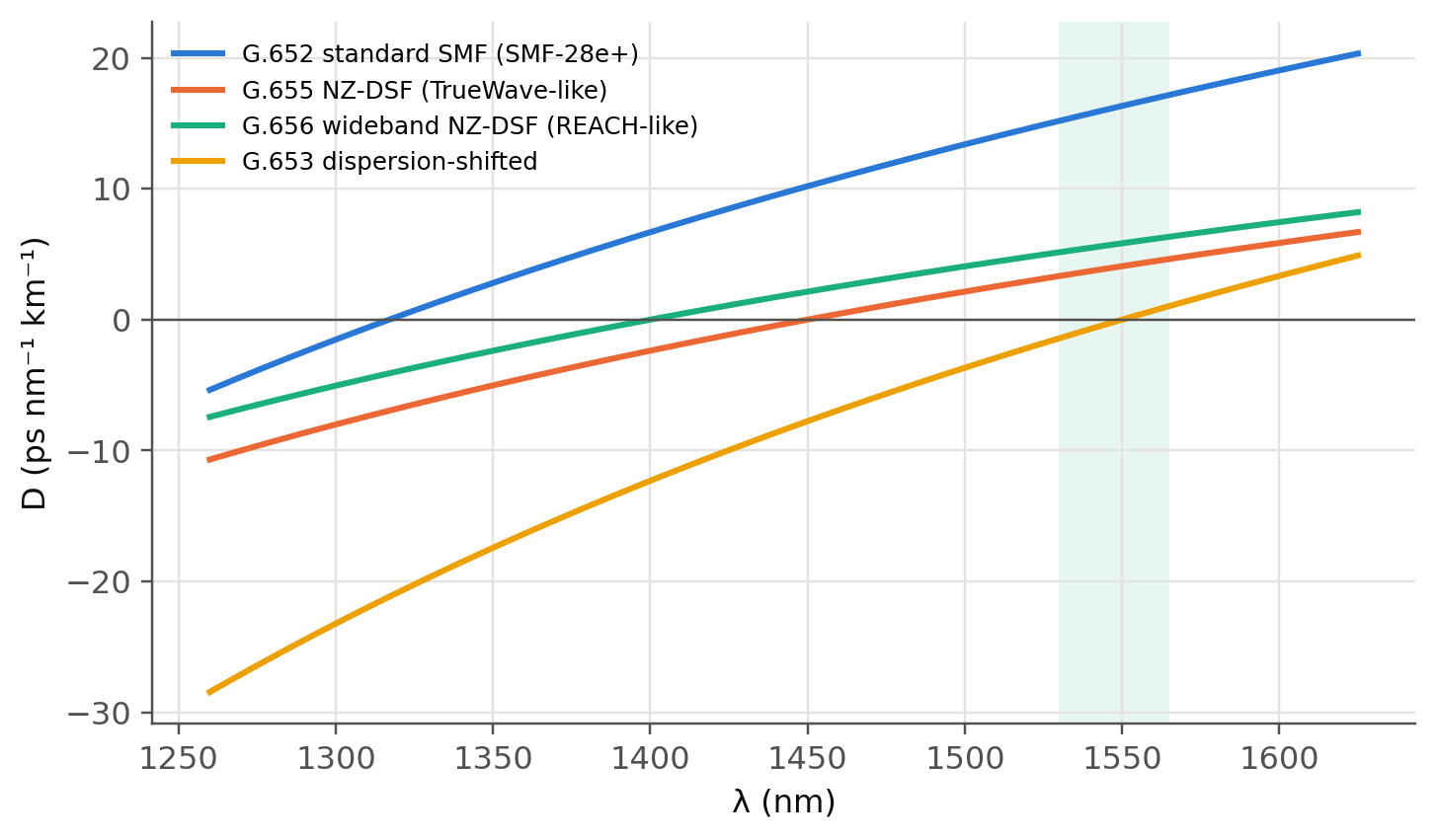
Near $\lambda_0$, the ITU-T recommendations describe $D(\lambda)$ with only two numbers, $\lambda_0$ and the slope $S_0$:
$$
D(\lambda)=\frac{S_0}{4}\left(\lambda-\frac{\lambda_0^4}{\lambda^3}\right).
$$
```{python}
#| label: fig-commercial
#| fig-cap: "Chromatic dispersion of typical commercial fibers described with the ITU formula. Values follow the table on slide 90 (G.652/SMF-28e+: λ0 = 1317 nm, S0 = 0.088). The NZ-DSF curves are representative."
lam = np.linspace(1260, 1625, 300)
fibs = {"G.652 standard SMF (SMF-28e+)": (1317, 0.088),
        "G.655 NZ-DSF (TrueWave-like)": (1450, 0.045),
        "G.656 wideband NZ-DSF (REACH-like)": (1400, 0.045),
        "G.653 dispersion-shifted": (1550, 0.07)}
fig, ax = plt.subplots()
for k, (name, (l0_, S0_)) in enumerate(fibs.items()):
    ax.plot(lam, S0_ / 4 * (lam - l0_**4 / lam**3), color=fl.PALETTE[k], label=name)
ax.axvspan(1530, 1565, color=fl.PALETTE[2], alpha=0.1, lw=0)
ax.axhline(0, color=fl.INK2, lw=0.8)
ax.set_xlabel("λ (nm)"); ax.set_ylabel("D (ps nm⁻¹ km⁻¹)"); ax.legend(fontsize=8)
plt.show()
```
## Is dispersion really zero at $\lambda_0$? (slide 79)
No. At $\lambda_0$ the first-order term vanishes, but the delay is still a **parabola** in $\lambda$:
$\tau(\lambda)\approx\tau_0+\tfrac{L S_0}{2}(\lambda-\lambda_0)^2$. The spread therefore scales as $\Delta\lambda^2$.
```{python}
L, S0_ = 100.0, 0.09          # km, ps/nm²/km
for dl in [0.1, 1, 2, 5, 10]:
    lin = 17 * L * dl
    quad = L * S0_ * dl**2 / 8          # spread over a ±Δλ/2 window around λ0
    print(f"Δλ = {dl:5.1f} nm : at 1550 nm {lin:9.1f} ps   |   at λ0 ≈ {quad:7.2f} ps")
```
## Polarisation mode dispersion (slides 80–83)
Random strains make the fiber weakly birefringent ($\delta n/n<10^{-6}$), with axes that rotate
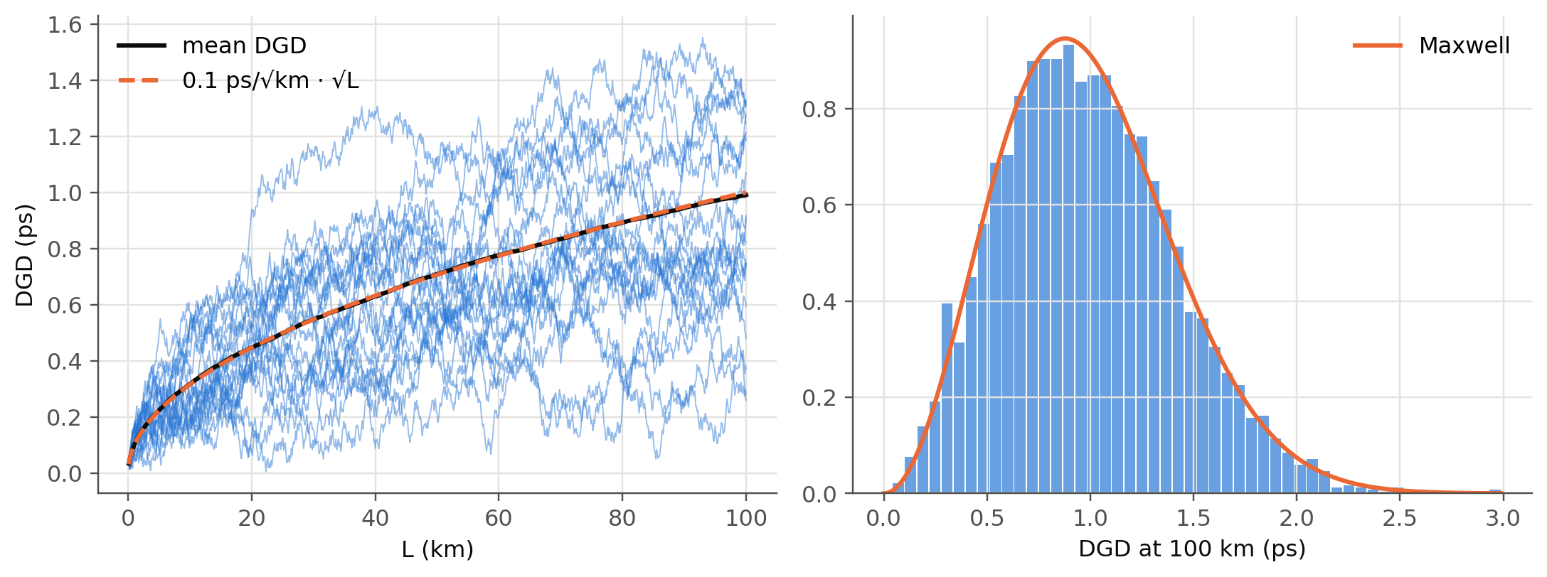
randomly along the length. The total differential group delay (DGD) is therefore a **random walk**.
The mean DGD grows as $\sqrt L$, $\langle\Delta\tau\rangle = D_\text{PMD}\sqrt L$, and its distribution is
**Maxwellian**. The concatenation rule for PMD vectors in Stokes space, $\vec\tau_{n+1}=R_n\vec\tau_n+\delta\vec\tau_n$,
with random rotations $R_n$, makes the vector perform a 3-D random walk:
```{python}
#| label: fig-pmd
#| fig-cap: "Monte-Carlo PMD. Left: DGD versus length for 20 random fibers (thin) and the ensemble mean ∝ √L. Right: histogram of the DGD at 100 km over 4000 fibers, with the Maxwell distribution."
rng = np.random.default_rng(3)
Lsec, nsec, nfib = 0.1, 1000, 4000            # 100 m sections, 100 km
dgd_sec = 0.1 / np.sqrt(1 / Lsec) * np.sqrt(3 * np.pi / 8)   # chosen so that <DGD> = 0.1 ps/√km
steps = rng.normal(size=(nfib, nsec, 3))
steps *= dgd_sec / np.linalg.norm(steps, axis=2, keepdims=True)
tau = np.linalg.norm(np.cumsum(steps, axis=1), axis=2)       # ps
z = np.arange(1, nsec + 1) * Lsec
fig, (a1, a2) = plt.subplots(1, 2, figsize=(10, 3.8))
a1.plot(z, tau[:20].T, color=fl.PALETTE[0], lw=0.6, alpha=0.5)
a1.plot(z, tau.mean(0), color=fl.INK, lw=2, label="mean DGD")
a1.plot(z, 0.1 * np.sqrt(z), "--", color=fl.PALETTE[1], label="0.1 ps/√km · √L")
a1.set_xlabel("L (km)"); a1.set_ylabel("DGD (ps)"); a1.legend()
t = tau[:, -1]; m = t.mean()
a2.hist(t, bins=50, density=True, color=fl.PALETTE[0], alpha=0.7, rwidth=0.9)
x = np.linspace(0, t.max(), 200)
a2.plot(x, 32 * x**2 / (np.pi**2 * m**3) * np.exp(-4 * x**2 / (np.pi * m**2)), color=fl.PALETTE[1], label="Maxwell")
a2.set_xlabel("DGD at 100 km (ps)"); a2.legend()
plt.tight_layout(); plt.show()
from scipy.special import erfc
s_ = m * np.sqrt(np.pi / 8)                    # Maxwell scale parameter
pmax = lambda x: erfc(x / (np.sqrt(2) * s_)) + np.sqrt(2 / np.pi) * x / s_ * np.exp(-x**2 / (2 * s_**2))
print(f"P(DGD > 2×mean): simulated {(t > 2*m).mean():.4f}, Maxwell {pmax(2*m):.4f}; "
      f"P(DGD > 3×mean) (Maxwell) = {pmax(3*m):.1e}. Outages are rare but not impossible.")
```
## Self-phase modulation: a first power limit (slide 86)
With $n'=n+CI$ and $C=10^{-14}$ cm²/W, which intensity gives $\Delta\tau/L\approx0.1$ ps/km?
$\Delta\tau/L = \Delta n/c$, so $\Delta n = c\,(0.1\text{ ps/km})$ and $I=\Delta n/C$.
```{python}
dn = c0 * 0.1e-12 / 1e3
I = dn / 1e-14                       # W/cm²
A = np.pi * (5e-4) ** 2               # cm², 2a = 10 µm
print(f"Δn = {dn:.1e},  I = {I:.1e} W/cm²,  A = {A:.2e} cm²,  P = I·A = {I*A:.2f} W in a 10 µm core")
```
This SPM-induced spread is small compared with chromatic dispersion. Other nonlinear effects (SBS, FWM; see
@sec-wdm) set in at much lower powers, at a few to a few tens of mW.
## Dispersion compensation (slides 93–95)
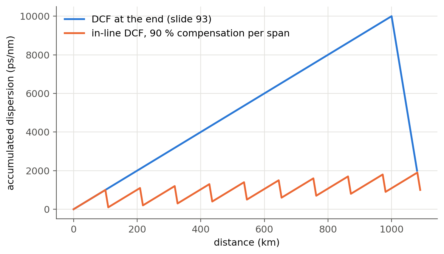
Add a short length $L_c$ of fiber with large dispersion of opposite sign, $D_c$. The accumulated dispersion is
$D_tL_t+D_cL_c$.
```{python}
#| label: fig-dmap
#| fig-cap: "Dispersion map. 1000 km of D = +10 ps/nm/km fiber with 80 km of D = −100 ps/nm/km DCF placed at the end (slide 93), compared with periodic in-line compensation every 100 km."
Dt, Dc = 10, -100
fig, ax = plt.subplots()
z = np.linspace(0, 1000, 500); ax.plot(np.r_[z, 1000 + np.linspace(0, 80, 50)],
        np.r_[Dt * z, Dt * 1000 + Dc * np.linspace(0, 80, 50)], label="DCF at the end (slide 93)")
zz, acc = [0], [0]
for span in range(10):
    zz += [zz[-1] + 100]; acc += [acc[-1] + Dt * 100]
    zz += [zz[-1] + 9.0]; acc += [acc[-1] + Dc * 9.0]
ax.plot(zz, acc, label="in-line DCF, 90 % compensation per span")
ax.set_xlabel("distance (km)"); ax.set_ylabel("accumulated dispersion (ps/nm)"); ax.legend()
plt.show()
print(f"Slide 93: total = {Dt*1000 + Dc*80} ps/nm over 1080 km → D_eff = {(Dt*1000 + Dc*80)/1080:.2f} ps/nm/km")
```
In modern **coherent** systems, compensation is done digitally in the receiver DSP
(see @sec-ideas). This removed DCFs from most new links.
## Try it yourself
1. Design a fiber with $\lambda_0=1550$ nm using the live panel. What happens to $V$ at 1.55 µm and to the MFD?
2. Using `fl.D_total_smf`, compute $D$ for a **W-profile (depressed cladding)**. You will need to extend the
solver to three layers. This is how *dispersion-flattened* fibers (slide 88) are made.
3. How many km of SMF can a 40 Gb/s NRZ signal travel if the tolerated spread is 0.3 bit periods,
with a 0.1 nm source? And with a source linewidth dominated by the modulation itself?