# WDM, couplers and nonlinear effects {#sec-wdm}
[](https://colab.research.google.com/github/{{< var github_user >}}/{{< var repo >}}/blob/main/{{< var subdir >}}/notebooks/wdm.ipynb){.colab-link} Run this chapter's code in Google Colab (no installation).
```{python}
#| include: false
import numpy as np
import matplotlib.pyplot as plt
import fiberlib as fl
fl.use_style()
c0, PS = fl.c0, fl.PS_NM_KM
```
*Slides 174–194.* One fiber, many colours. Wavelength-division multiplexing (WDM) multiplies the capacity of a
fiber by the number of channels, but it brings new problems: components that combine and split light, and
nonlinear interactions between channels.
## The ITU grid (slides 175–176)
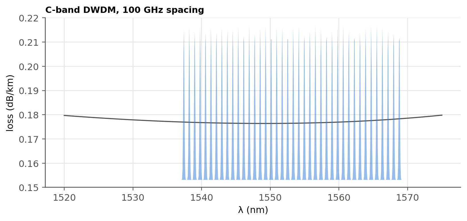
DWDM channels sit on a frequency grid anchored at 193.1 THz. A channel spacing $\Delta\nu$ corresponds to
$\Delta\lambda=\lambda^2\Delta\nu/c$.
```{python}
for dnu in [200, 100, 50, 12.5]:
    print(f"Δν = {dnu:6.1f} GHz  ↔  Δλ = {(1.55e-6)**2*dnu*1e9/c0*1e9:.3f} nm at 1550 nm;  "
          f"channels in the C-band (4.4 THz): {int(4.4e3/dnu)}")
```
```{python}
#| label: fig-grid
#| fig-cap: "40 DWDM channels on the 100 GHz ITU grid across the C-band, drawn over the fiber loss. Each channel carries its own data stream (e.g. 100 Gb/s → 4 Tb/s per fiber)."
nu = 193.1e12 + np.arange(-20, 20) * 100e9
lam_ch = c0 / nu
lam = np.linspace(1520, 1575, 800) * 1e-9
fig, ax = plt.subplots(figsize=(8.5, 3.5))
ax.plot(lam * 1e9, fl.attenuation_model(lam, OH_peak=0), color=fl.INK2, lw=1.2, label="fiber loss (dB/km)")
ax2 = ax.twinx(); ax2.grid(False)
spec = sum(np.exp(-0.5 * ((lam - l) / 0.08e-9) ** 2) for l in lam_ch)
ax2.fill_between(lam * 1e9, spec, color=fl.PALETTE[0], alpha=0.5, lw=0)
ax2.set_yticks([]); ax2.spines["right"].set_visible(False)
ax.set_xlabel("λ (nm)"); ax.set_ylabel("loss (dB/km)"); ax.set_ylim(0.15, 0.22)
ax.set_title("C-band DWDM, 100 GHz spacing", loc="left", fontsize=10)
plt.show()
```
## Passive couplers (slides 177–184)
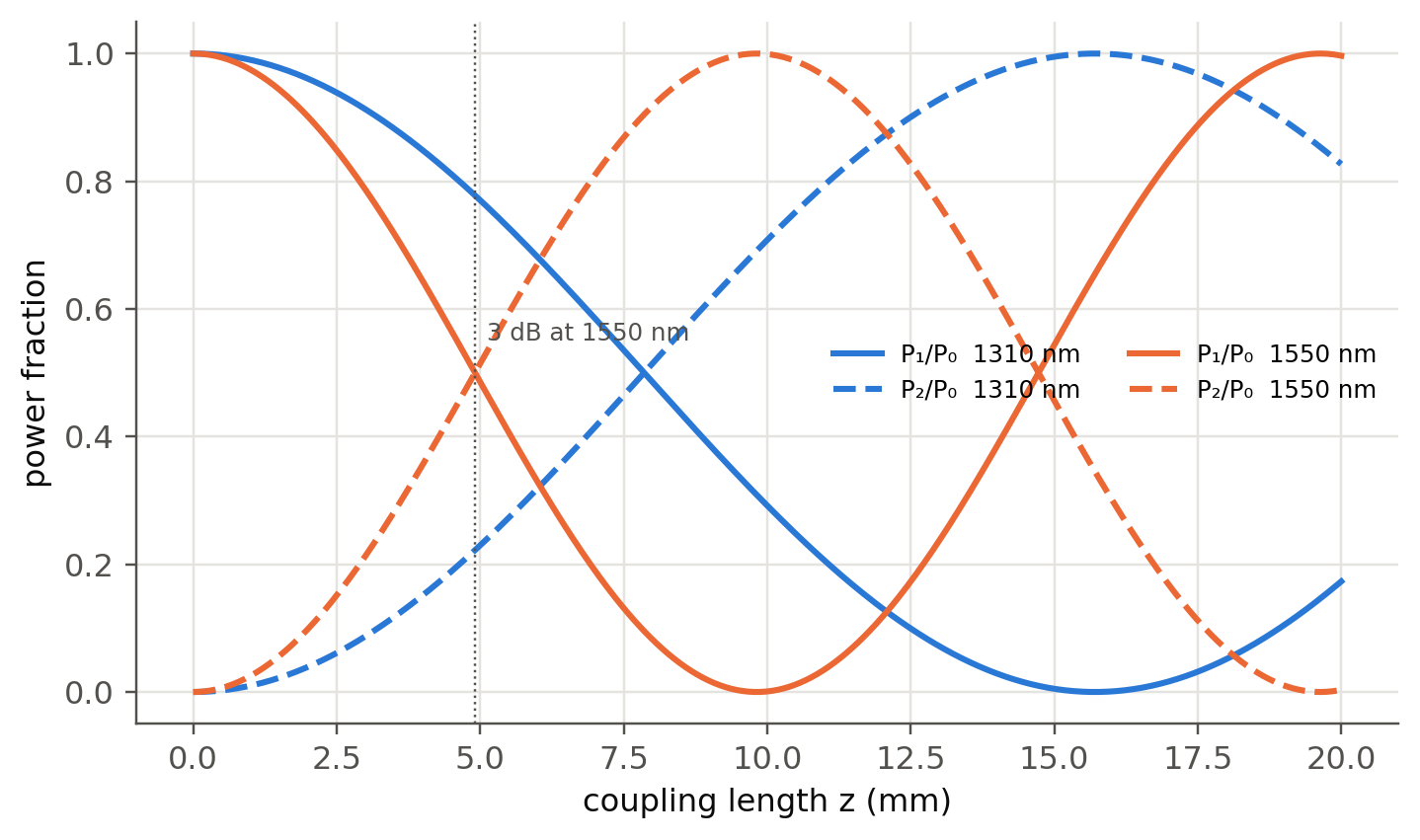
In a fused 2×2 coupler the evanescent tail of one core excites the other (slide 178). Coupled-mode theory gives a
periodic exchange of power along the coupling length $z$:
$$
P_1=P_0\cos^2(\kappa z),\qquad P_2=P_0\sin^2(\kappa z).
$$
```{python}
#| label: fig-coupler
#| fig-cap: "Power exchange in a symmetric directional coupler. A 3 dB coupler needs κz = π/4. The coupling coefficient depends on wavelength, so a coupler designed for 1310 nm splits 1550 nm differently. This is the basis of the 1310/1550 WDM coupler."
z = np.linspace(0, 20, 400)                  # mm
fig, ax = plt.subplots()
for k, (lam, kap) in enumerate([(1310, 0.10), (1550, 0.16)]):
    ax.plot(z, np.cos(kap * z) ** 2, color=fl.PALETTE[k], label=f"P₁/P₀  {lam} nm")
    ax.plot(z, np.sin(kap * z) ** 2, "--", color=fl.PALETTE[k], label=f"P₂/P₀  {lam} nm")
ax.axvline(np.pi / 4 / 0.16, color=fl.INK2, lw=0.8, ls=":")
ax.text(np.pi / 4 / 0.16 + 0.2, 0.55, "3 dB at 1550 nm", color=fl.INK2, fontsize=8)
ax.set_xlabel("coupling length z (mm)"); ax.set_ylabel("power fraction"); ax.legend(ncol=2, fontsize=8)
plt.show()
```
The performance figures (slide 179) are, in dB:
| figure | definition | 3 dB coupler | tap coupler |
|---|---|---|---|
| split ratio | $P_2/(P_1+P_2)$ | 50 % | 0.5 % |
| excess loss | $10\log\frac{P_0}{P_1+P_2}$ | ~0.1 dB | ~0.1 dB |
| insertion loss | $10\log\frac{P_0}{P_j}$ | ~3.1 dB | ~23 dB (tap port) |
| crosstalk / directivity | $10\log\frac{P_3}{P_0}$ | −50 to −70 dB | |
### Star couplers
An $N\times N$ star built from 3 dB couplers needs $\frac N2\log_2N$ couplers, and each output gets $1/N$ of the
power. That is a splitting loss of $10\log_{10}N$ dB, plus the excess loss of each stage.
```{python}
for N in [2, 4, 8, 16, 32, 64]:
    st = int(np.log2(N))
    print(f"N = {N:3d}: {N//2*st:4d} couplers, {st} stages, splitting loss {10*np.log10(N):5.1f} dB, "
          f"with 0.1 dB excess/stage: {10*np.log10(N)+0.1*st:5.1f} dB")
```
This is the architecture of a **passive optical network (PON)** that brings fiber to the home: one 1×32 or 1×64
splitter feeds many households.
## Four-wave mixing (slides 185–188)
The third-order polarisation $P\propto a_3E^3$ mixes three channels $\nu_i,\nu_j,\nu_k$ into new frequencies
$$
\nu_{ijk}=\nu_i+\nu_j-\nu_k .
$$
With **equally spaced** channels, many products fall **exactly on top of existing channels** and become crosstalk
that cannot be filtered. With $N$ channels there are $N^2(N-1)/2$ products.
```{ojs}
//| echo: false
viewof fwm = Inputs.form({
  N: Inputs.range([3, 16], {value: 8, step: 1, label: "number of channels"}),
  sp: Inputs.radio(["equal", "unequal (Golomb-like)"], {value: "equal", label: "spacing"})
})
```
```{ojs}
//| echo: false
fwmData = {
  const golomb = [0, 1, 4, 9, 15, 22, 32, 34, 49, 55, 72, 86, 106, 114, 126, 149];
  const ch = d3.range(fwm.N).map(i => fwm.sp === "equal" ? i : golomb[i] * 0.55);
  const prods = new Map();
  for (const i of ch) for (const j of ch) for (const k of ch) {
    if (k === i || k === j) continue;
    if (j < i) continue;               // ν_i + ν_j symmetric
    const f = +(i + j - k).toFixed(3);
    prods.set(f, (prods.get(f) || 0) + 1);
  }
  const P = [...prods].map(([f, n]) => ({f, n, onChannel: ch.some(c => Math.abs(c - f) < 1e-6)}));
  return {ch, P, hits: d3.sum(P.filter(d => d.onChannel), d => d.n), total: d3.sum(P, d => d.n)};
}
Plot.plot({
  width: Math.min(width, 1050), height: 260, x: {label: "frequency (units of spacing)"}, y: {label: "number of FWM products", grid: true},
  color: {domain: [true, false], range: ["#e34948", "#b9b8b2"], legend: true, tickFormat: d => d ? "falls on a channel" : "between channels"},
  marks: [
    Plot.ruleX(fwmData.ch, {stroke: "#2a78d6", strokeWidth: 3, y1: 0, y2: d3.max(fwmData.P, d => d.n) * 1.1}),
    Plot.ruleX(fwmData.P, {x: "f", y: "n", stroke: "onChannel", strokeWidth: 2}),
    Plot.dot(fwmData.P, {x: "f", y: "n", fill: "onChannel", r: 3, tip: true, title: d => `ν = ${d.f}\n${d.n} products`})
  ]
})
```
```{ojs}
//| echo: false
html`<div class="result-box">${fwm.N} channels (blue) → ${fwmData.total} mixing products (N²(N−1)/2 = ${fwm.N**2*(fwm.N-1)/2}),
of which <b>${fwmData.hits}</b> fall exactly on a signal channel.</div>`
```
### Why a little dispersion helps (slide 87)
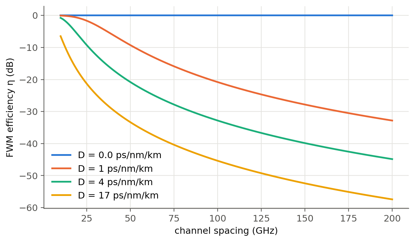
FWM needs **phase matching**. The mismatch $\Delta\beta\approx\frac{2\pi\lambda^2}{c}D\,\Delta\nu^2$ grows with $D$. The
efficiency $\eta\approx\frac{\alpha^2}{\alpha^2+\Delta\beta^2}$ drops quickly when the channels walk off from each other.
This is the reason for **non-zero** dispersion-shifted fibers.
```{python}
#| label: fig-fwm-eta
#| fig-cap: "Approximate FWM efficiency versus channel spacing for fibers with different dispersion (α = 0.2 dB/km). At D = 0 (DSF) FWM is phase-matched for every spacing. A few ps/nm/km (NZ-DSF) is enough to suppress it."
dnu = np.linspace(10e9, 200e9, 400)
alpha = 0.2 / 4.343 / 1e3
fig, ax = plt.subplots()
for k, D in enumerate([0.0, 1, 4, 17]):
    db = 2 * np.pi * (1.55e-6) ** 2 / c0 * D * PS * dnu**2
    ax.plot(dnu / 1e9, 10 * np.log10(alpha**2 / (alpha**2 + db**2)), color=fl.PALETTE[k], label=f"D = {D} ps/nm/km")
ax.set_xlabel("channel spacing (GHz)"); ax.set_ylabel("FWM efficiency η (dB)"); ax.legend()
plt.show()
```
## Self-phase modulation and chirp (slides 189–190)
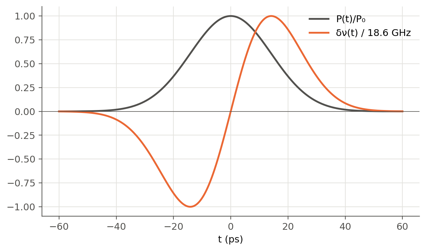
With $n=n_0+n_2I$, a pulse modulates its own phase, $\phi_{NL}(t)=-\gamma P(t)L_\text{eff}$. The instantaneous
frequency shift is $\delta\omega=-d\phi_{NL}/dt$: red on the leading edge, blue on the trailing edge.
```{python}
#| label: fig-spm
#| fig-cap: "SPM-induced chirp of a 20 ps Gaussian pulse (peak 100 mW, γ = 1.3 /W/km, L_eff = 21 km)."
t = np.linspace(-60, 60, 600) * 1e-12
T0, P0, gam, Leff = 20e-12, 0.1, 1.3e-3, 21e3
P = P0 * np.exp(-(t / T0) ** 2)
phi = gam * P * Leff
dnu = -np.gradient(phi, t) / (2 * np.pi)
fig, ax = plt.subplots()
ax.plot(t * 1e12, P / P0, color=fl.INK2, label="P(t)/P₀")
ax.plot(t * 1e12, dnu / np.abs(dnu).max(), color=fl.PALETTE[1], label=f"δν(t) / {np.abs(dnu).max()/1e9:.1f} GHz")
ax.axhline(0, color=fl.INK2, lw=0.6)
ax.set_xlabel("t (ps)"); ax.legend(); plt.show()
print(f"Max nonlinear phase = {phi.max():.2f} rad")
```
## Stimulated Brillouin scattering (slides 191–194)
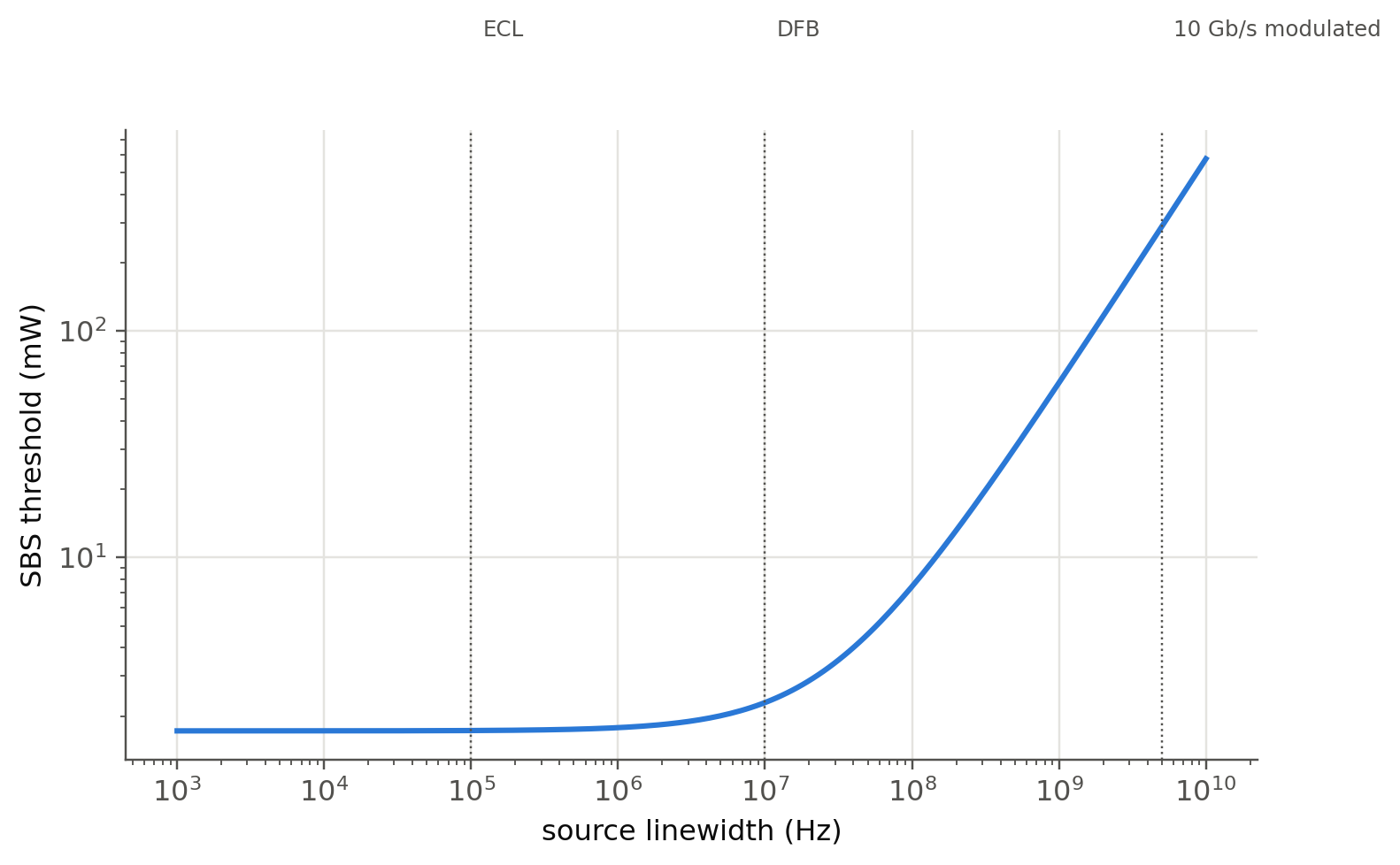
A narrow-line, high-power signal is reflected back by the acoustic grating it creates itself. A classic estimate of
the threshold is
$$
P_\text{th}\approx21\frac{A_\text{eff}}{g_BL_\text{eff}}\left(1+\frac{\Delta\nu_s}{\Delta\nu_B}\right),\qquad
L_\text{eff}=\frac{1-e^{-\alpha L}}{\alpha},
$$
with $g_B\approx5\times10^{-11}$ m/W and a Brillouin linewidth $\Delta\nu_B\approx30$ MHz.
```{python}
#| label: fig-sbs
#| fig-cap: "SBS threshold versus source linewidth for SMF (A_eff = 80 µm²) over 50 km. A narrow external-cavity laser (kHz–MHz) hits SBS at a few mW. Broadening the line (dithering, modulation) pushes the threshold up."
Aeff, gB, dnB = 80e-12, 5e-11, 30e6
Leff = (1 - np.exp(-alpha * 50e3)) / alpha
lw = np.logspace(3, 10, 200)
Pth = 21 * Aeff / (gB * Leff) * (1 + lw / dnB)
fig, ax = plt.subplots()
ax.loglog(lw, Pth * 1e3)
for x, txt in [(1e5, "ECL"), (1e7, "DFB"), (5e9, "10 Gb/s modulated")]:
    ax.axvline(x, color=fl.INK2, lw=0.8, ls=":"); ax.text(x * 1.2, 2e3, txt, color=fl.INK2, fontsize=8)
ax.set_xlabel("source linewidth (Hz)"); ax.set_ylabel("SBS threshold (mW)")
plt.show()
print(f"L_eff = {Leff/1e3:.1f} km; narrow-line threshold ≈ {21*Aeff/(gB*Leff)*1e3:.1f} mW")
```
## Try it yourself
1. Extend the FWM panel to compute the **power** of each product,
$P_{ijk}\propto\eta\,(D_{ijk}\gamma L_\text{eff})^2P_iP_jP_k$ (degeneracy factor $D_{ijk}=3$ or 6), and the resulting
SNR on the worst channel.
2. Design an unequal channel plan for 8 channels in which **no** product falls on a channel, with the smallest
total bandwidth. (Hint: Golomb rulers.)
3. Implement the **split-step Fourier method** (a ~20-line loop alternating `fl.imdd_link`-style linear steps and
$e^{j\gamma|E|^2h}$) and observe SPM-induced spectral broadening and soliton formation for $D>0$.